8 8 0 0 Total (X-X)2 = 4 + 0 + 16 + 36 + 0 = 56 n-1 = 5 - 1 = 4 S = √(Total (X-X)2 / (n-1)) = √(56/4) = √14 = 3.74 Therefore, the standard deviation of returns on Stock X is 3.74%

1. What is
Business
Statistics?

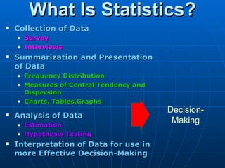
3. What Is Statistics?
 Collection of Data
• Survey
• Interviews
 Summarization and Presentation
of Data
• Frequency Distribution
• Measures of Central Tendency and
Dispersion
• Charts, Tables,Graphs
Decision-
 Analysis of Data
• Estimation
Making
• Hypothesis Testing
 Interpretation of Data for use in
more Effective Decision-Making

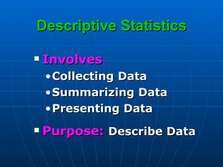
4. Descriptive Statistics
 Involves
• Collecting Data
• Summarizing Data
• Presenting Data
 Purpose: Describe Data

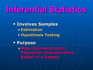
5. Inferential Statistics
 Involves Samples
• Estimation
• Hypothesis Testing
 Purpose
• Make Decisions About
Population Characteristics
Based on a Sample

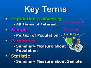
6. Key Terms
 Population (Universe)
• P in Population
• All Items of Interest
 Sample & Parameter
• Portion of Population • S in Sample
& Statistic
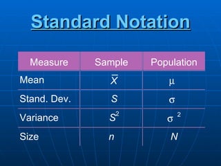
 Parameter
• Summary Measure about
Population
 Statistic
• Summary Measure about Sample

7. Collection
of
Data

8. Data Types
 Quantitative (categorical)
 Qualitative (numerical)
• Discrete
• Continuous

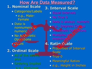
9. How Are Data Measured?
1. Nominal Scale 3. Interval Scale
• Categories/Labels
• Equal Intervals
 e.g., Male-
• No True 0
Female
• Data is always numeric
• Data is
nonnumeric or
v e • e.g., Degrees Celsius
v e
numeric
ti ti
• Arithmetic Operations
ta
i ta
• No Arithmetic
l ti
• Multiples not
a
Operations n
meaningful
a
u
• Count u
4. Ratio Scale
Q Q
• Properties of Interval
2. Ordinal Scale Scale
• All of the above, • True 0
plus
• Meaningful Ratios
• Ordering Implied
• e.g., Height in Inches

10. Summarization
and
Presentation
of
Data

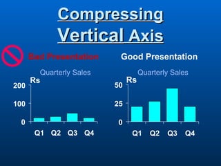
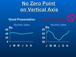
11. Data Presentation
 Ordered Array
 Stem and Leaf Display
 Frequency Distribution
• Histogram
• Polygon
• Ogive

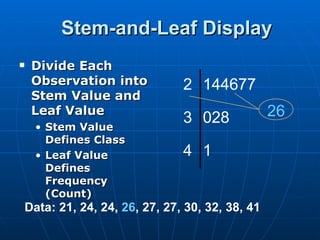
12. Stem-and-Leaf Display
 Divide Each
Observation into 2 144677
Stem Value and
Leaf Value
3 028 26
• Stem Value
Defines Class
• Leaf Value 4 1
Defines
Frequency
(Count)
Data: 21, 24, 24, 26, 27, 27, 30, 32, 38, 41

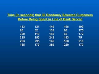
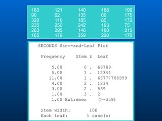
13. Time (in seconds) that 30 Randomly Selected Customers
Before Being Spent in Line of Bank Served
183 121 140 198 199
90 62 135 60 175
320 110 185 85 172
235 250 242 193 75
263 295 146 160 210
165 179 359 220 170

14. 183 121 140 198 199
90 62 135 60 175
320 110 185 85 172
235 250 242 193 75
263 295 146 160 210
165 179 359 220 170
SECONDS Stem-and-Leaf Plot
Frequency Stem & Leaf
5.00 0 . 66789
5.00 1 . 12344
11.00 1 . 66777788999
4.00 2 . 1234
3.00 2 . 569
1.00 3 . 2
1.00 Extremes (>=359)
Stem width: 100
Each leaf: 1 case(s)

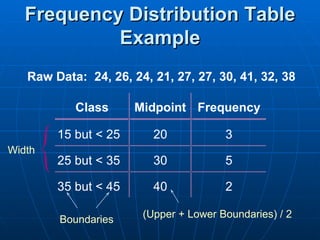
15. Frequency Distribution Table
Example
Raw Data: 24, 26, 24, 21, 27, 27, 30, 41, 32, 38
Class Midpoint Frequency
15 but < 25 20 3
Width
25 but < 35 30 5
35 but < 45 40 2
(Upper + Lower Boundaries) / 2
Boundaries

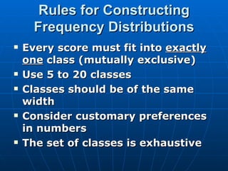
16. Rules for Constructing
Frequency Distributions
 Every score must fit into exactly
one class (mutually exclusive)
 Use 5 to 20 classes
 Classes should be of the same
width
 Consider customary preferences
in numbers
 The set of classes is exhaustive

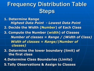
17. Frequency Distribution Table
Steps
1. Determine Range
Highest Data Point - Lowest Data Point
2. Decide the Width (Number) of Each Class
3. Compute the Number (width) of Classes
Number of classes = Range / (Width of Class)
Width of classes = Range/(Number of
classes)
3. Determine the lower boundary (limit) of
the first class
4. Determine Class Boundaries (Limits)
5. Tally Observations & Assign to Classes

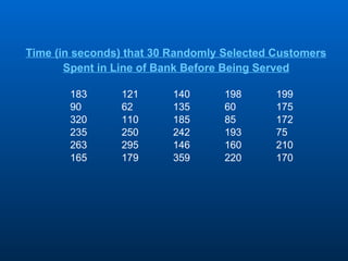
18. Time (in seconds) that 30 Randomly Selected Customers
Spent in Line of Bank Before Being Served
183 121 140 198 199
90 62 135 60 175
320 110 185 85 172
235 250 242 193 75
263 295 146 160 210
165 179 359 220 170

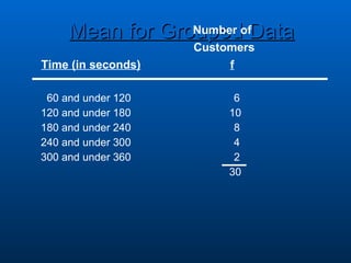
19. Mean for GroupedofData
Number
Customers
Time (in seconds) f
60 and under 120 6
120 and under 180 10
180 and under 240 8
240 and under 300 4
300 and under 360 2
30

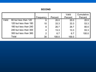
20. SECOND
Valid Cumulative
Frequency Percent Percent Percent
Valid 60 but less than 120 6 20.0 20.0 20.0
120 but less than 180 10 33.3 33.3 53.3
180 but less than 240 8 26.7 26.7 80.0
240 but less than 300 4 13.3 13.3 93.3
300 but less than 360 2 6.7 6.7 100.0
Total 30 100.0 100.0

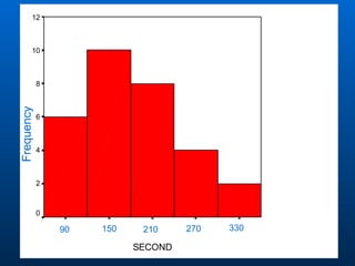
21. 12
10
8
Frequency
6
4
2 Std. Dev = 1.17
Mean = 3
0 N = 30.00
1 2 3 4 5
90 150 210 270 330
SECOND

22. ‘Chart Junk’
Bad Presentation Good Presentation
Minimum Wage Minimum Wage
1960: Rs1.00 Rs
4
1970: Rs1.60
2
1980: Rs3.10
0
1990: Rs.3.80 1960 1970 1980 1990

23. No Relative Basis
Bad Presentation Good Presentation
A’s by Class A’s by Class
Freq. %
300 30%
200 20%
100 10%
0 0%
FR SO JR SR FR SO JR SR

24. Compressing
Vertical Axis
Bad Presentation Good Presentation
Quarterly Sales Quarterly Sales
Rs Rs
200 50
100 25
0 0
Q1 Q2 Q3 Q4 Q1 Q2 Q3 Q4

25. No Zero Point
on Vertical Axis
Good Presentation Bad Presentation
Monthly Sales Monthly Sales
Rs Rs
60 45
40 42
20 39
0 36
J M M J S N J M M J S N

26. Standard Notation
Measure Sample Population
Mean X µ
Stand. Dev. S σ
2 2
Variance S σ
Size n N

27. Numerical Data
Properties
Central Tendency
(Location)
Variation
(Dispersion)
Shape

28. Measures of Central
Tendency
for
Ungrouped Data
Raw Data

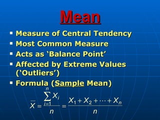
29. Mean
 Measure of Central Tendency
 Most Common Measure
 Acts as ‘Balance Point’
 Affected by Extreme Values
(‘Outliers’)
 Formula (Sample Mean)
n
∑ Xi X1 + X 2 +  + X n
i =1
X= =
n n

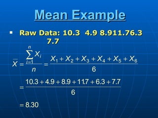
30. Mean Example
 Raw Data: 10.3 4.9 8.911.76.3
7.7
n
∑ Xi X1 + X 2 + X 3 + X 4 + X 5 + X 6
i =1
X= =
n 6
10.3 + 4.9 + 8.9 + 117 + 6.3 + 7.7
.
=
6
= 8.30

31. Advantages of the Mean
 Most widely used
 Every item taken into account
 Determined algebraically and
amenable to algebraic
operations
 Can be calculated on any set of
numerical data (interval and
ratio scale) -Always exists
 Unique
 Relatively reliable

32. Disadvantages of
the Mean
 Affected by outliers
 Cannot use in open-
ended classes of a
frequency distribution

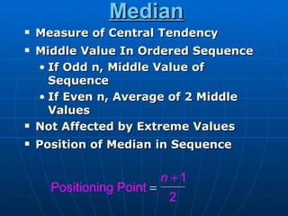
33. Median
 Measure of Central Tendency
 Middle Value In Ordered Sequence
• If Odd n, Middle Value of
Sequence
• If Even n, Average of 2 Middle
Values
 Not Affected by Extreme Values
 Position of Median in Sequence
n +1
Positioning Point =
g
2

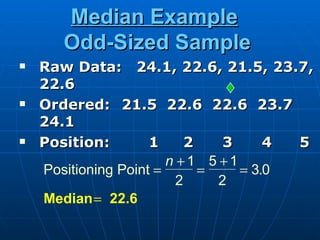
34. Median Example
Odd-Sized Sample
 Raw Data: 24.1, 22.6, 21.5, 23.7,
22.6
 Ordered: 21.5 22.6 22.6 23.7
24.1
 Position: 1 2 3 4 5
n +1 5 +1
Positioning Point = = = 3.0
2 2
Median = 22.6

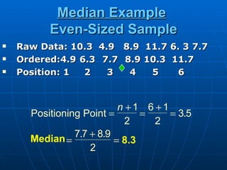
35. Median Example
Even-Sized Sample
 Raw Data: 10.3 4.9 8.9 11.7 6. 3 7.7
 Ordered:4.9 6.3 7.7 8.9 10.3 11.7
 Position: 1 2 3 4 5 6
n +1 6 +1
Positioning Point = = = 3.5
2 2
Median = 7.7 + 8.9
= 8.3
2

36. Advantages of the Median
 Unique
 Unaffected by outliers and
skewness
 Easily understood
 Can be computed for open-
ended classes of a frequency
distribution
 Always exists on ungrouped
data
 Can be computed on ratio,
interval and ordinal scales

37. Disadvantages of
Median
 Requires an ordered array
 No arithmetic properties

38. Mode
 Measure of Central Tendency
 Value That Occurs Most Often
 Not Affected by Extreme Values
 May Be No Mode or Several
Modes
 May Be Used for Numerical &
Categorical Data

39. Advantages of Mode
 Easily understood
 Not affected by outliers
 Useful with qualitative
problems
 May indicate a bimodal
distribution

40. Disadvantages of
Mode
 May not exist
 Not unique
 No arithmetic
properties
 Least accurate

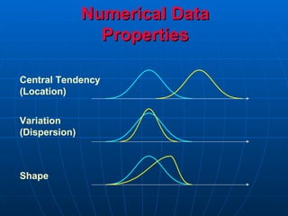
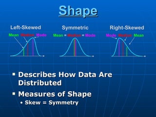
41. Shape
Left-Skewed Symmetric Right-Skewed
Mean Median Mode Mean = Median = Mode Mode Median Mean
 Describes How Data Are
Distributed
 Measures of Shape
• Skew = Symmetry

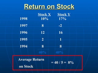
42. Return on Stock
Stock X Stock Y
1998 10% 17%
1997 8 -2
1996 12 16
1995 2 1
1994 8 8
40% 40%
Average Return
= 40 / 5 = 8%
on Stock

43. Measures of
Dispersion
for
Ungrouped Data
Raw Data

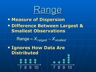
44. Range
 Measure of Dispersion
 Difference Between Largest &
Smallest Observations
Range = X l arg est − X smallest
 Ignores How Data Are
Distributed
7 8 9 10 7 8 9 10

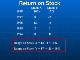
45. Return on Stock
Stock X Stock Y
1998 10% 17%
1997 8 -2
1996 12 16
1995 2 1
1994 8 8
Range on Stock X = 12 - 2 = 10%
Range on Stock Y = 17 - (-2) = 19%

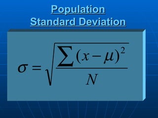
46. Variance &
Standard Deviation
 Measures of Dispersion
 Most Common Measures
 Consider How Data Are
Distributed
 Show Variation About Mean ( X
or µ )

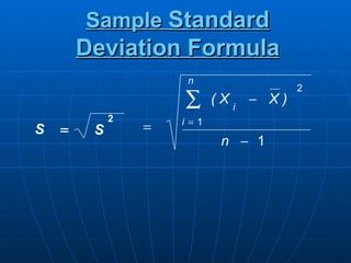
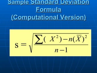
47. Sample Standard
Deviation Formula
n
2
∑ (Xi − X)
2 i =1
S = S =
n − 1

48. Sample Standard Deviation
Formula
(Computational Version)
s= ∑( X ) − n( X )
2 2
n −1

49. Return on Stock
Stock X Stock Y
1998 10% 17%
1997 8 -2
1996 12 16
1995 2 1
1994 8 8
Range on Stock X = 12 - 2 = 10%
Range on Stock Y = 17 - (-2) = 19%

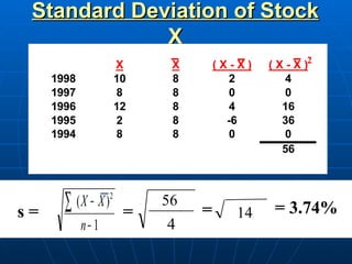
50. Standard Deviation of Stock
X
X X (X-X) ( X - X )2
1998 10 8 2 4
1997 8 8 0 0
1996 12 8 4 16
1995 2 8 -6 36
1994 8 8 0 0
56
s= ∑ (X − X ) 2
=
56
= 14 = 3.74%
n− 1 4

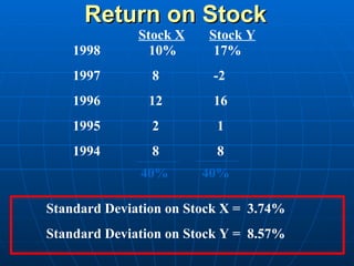
51. Return on Stock
Stock X Stock Y
1998 10% 17%
1997 8 -2
1996 12 16
1995 2 1
1994 8 8
40% 40%
Standard Deviation on Stock X = 3.74%
Standard Deviation on Stock Y = 8.57%

52. Population Mean
µ= ∑ x
N

53. Population
Standard Deviation
σ= ∑ (x − µ) 2
N

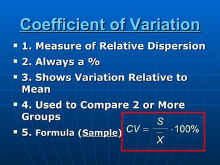
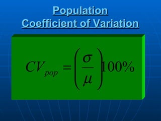
54. Coefficient of Variation
 1. Measure of Relative Dispersion
 2. Always a %
 3. Shows Variation Relative to
Mean
 4. Used to Compare 2 or More
Groups S
 5. Formula (Sample) CV = ⋅100%
X

55. Population
Coefficient of Variation
σ 
CV pop =  100%
µ
 

56. Example
You’re a financial analyst for Prudential-
Bache Securities. You have also collected the
closing stock prices of 20 old stock issues
and determined the mean price is Rs.10.89
and the standard deviation was Rs.3.95.
Which stock prices - old or new- were
relatively more variable?

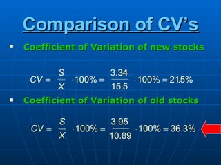
57. Comparison of CV’s
 Coefficient of Variation of new stocks
S 3.34
34
CV = ⋅ 100% = ⋅ 100% = 215%
.
X 15.5
 Coefficient of Variation of old stocks
S 3.95
CV = ⋅ 100% = ⋅ 100% = 36.3%
X 10.89