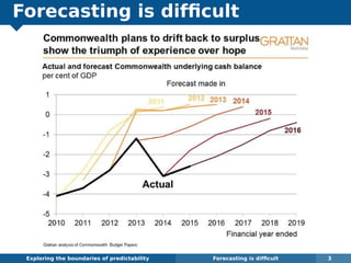
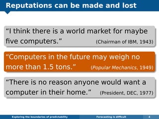
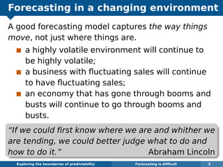
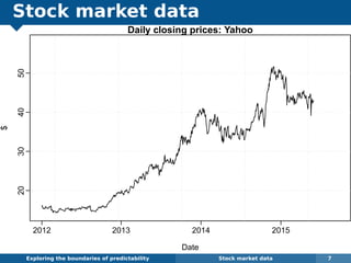
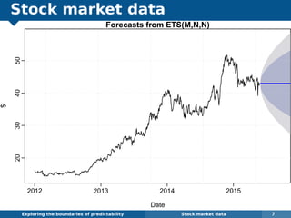
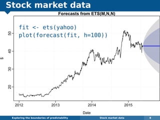
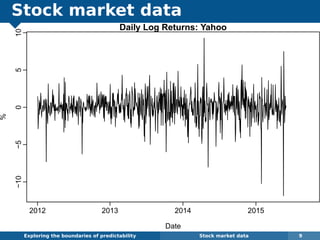
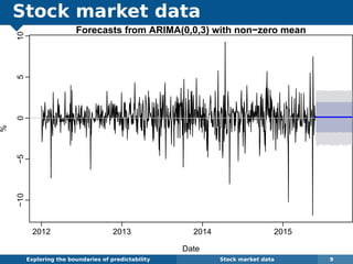
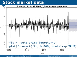
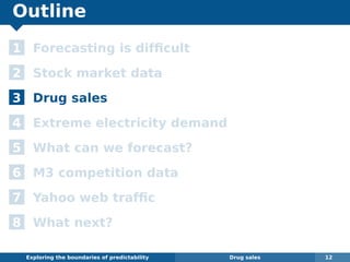
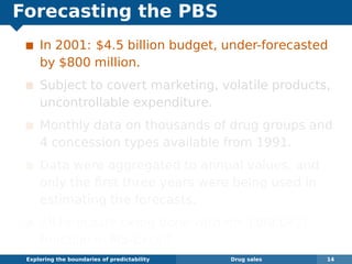
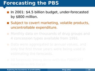
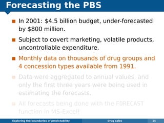
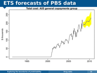
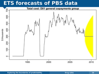
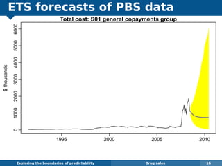
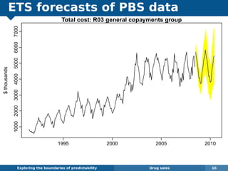
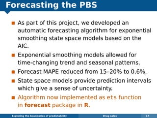
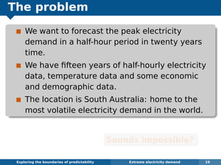
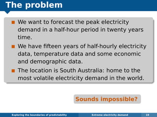
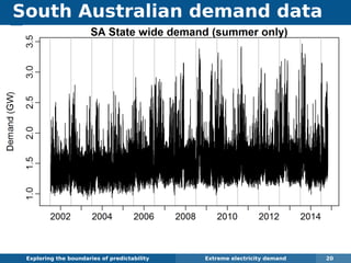
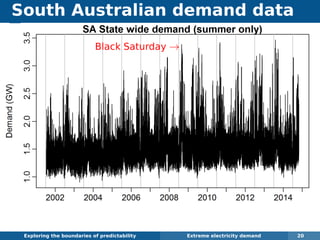
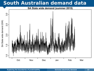
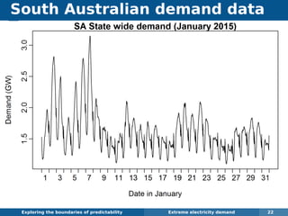
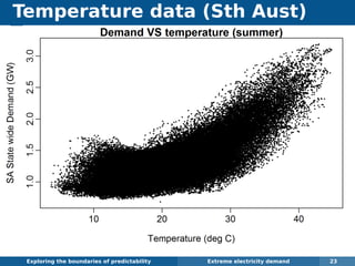
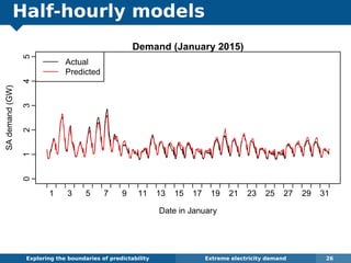
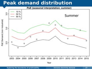
Why is it that we can accurately forecast a solar eclipse in 1000 years time, but we have no idea whether Yahoo's stock price will rise or fall tomorrow? Or why can we forecast electricity consumption next week with remarkable precision, but we cannot forecast exchange rate fluctuations in the next hour?
In this talk, I will discuss the conditions we need for predictability, how to measure the uncertainty of predictions, and the consequences of thinking we can predict something more accurately than we can.
I will draw on my experiences in forecasting Australia's health budget for the next few years, in developing forecasting models for peak electricity demand in 20 years time, and in identifying unpredictable activity on Yahoo's mail servers.
Automatic algorithms for time series forecastingRob Hyndman
Many applications require a large number of time series to be forecast completely automatically. For example, manufacturing companies often require weekly forecasts of demand for thousands of products at dozens of locations in order to plan distribution and maintain suitable inventory stocks. In these circumstances, it is not feasible for time series models to be developed for each series by an experienced analyst. Instead, an automatic forecasting algorithm is required.
In addition to providing automatic forecasts when required, these algorithms also provide high quality benchmarks that can be used when developing more specific and specialized forecasting models.
I will describe some algorithms for automatically forecasting univariate time series that have been developed over the last 20 years. The role of forecasting competitions in comparing the forecast accuracy of these algorithms will also be discussed.
Exploring the feature space of large collections of time seriesRob Hyndman
It is becoming increasingly common for organizations to collect very large amounts of data over time. Data visualization is essential for exploring and understanding structures and patterns, and to identify unusual observations. However, the sheer quantity of data available challenges current time series visualisation methods.
For example, Yahoo has banks of mail servers that are monitored over time. Many measurements on server performance are collected every hour for each of thousands of servers. We wish to identify servers that are behaving unusually.
Alternatively, we may have thousands of time series we wish to forecast, and we want to be able to identify the types of time series that are easy to forecast and those that are inherently challenging.
I will demonstrate a functional data approach to this problem using a vector of features on each time series, measuring characteristics of the series. For example, the features may include lag correlation, strength of seasonality, spectral entropy, etc. Then we use a principal component decomposition on the features, and plot the first few principal components. This enables us to explore a lower dimensional space and discover interesting structure and unusual observations.
MEFM: An R package for long-term probabilistic forecasting of electricity demandRob Hyndman
I will describe and demonstrate a new open-source R package that implements the Monash Electricity Forecasting Model, a semi-parametric probabilistic approach to forecasting long-term electricity demand. The underlying model proposed in Hyndman and Fan (2010) is now widely used in practice, particularly in Australia. The model has undergone many improvements and developments since it was first proposed, and these have been incorporated in this R implementation.
The package allows for ensemble forecasting of demand based on simulations of future sample paths of temperatures and other predictor variables. It requires the following data as inputs: half-hourly/hourly electricity demands; half-hourly/hourly temperatures at one or two locations; seasonal (e.g., quarterly) demographic and economic data; and public holiday data.
Peak electricity demand forecasting is important in medium and long-term planning of electricity supply. Extreme demand often leads to supply failure with consequential business and social disruption. Forecasting extreme demand events is therefore an important problem in energy management, and this package provides a useful tool for energy companies and regulators in future planning.
Forecasting electricity demand distributions using a semiparametric additive ...Rob Hyndman
Electricity demand forecasting plays an important role in short-term load allocation and long-term planning for future generation facilities and transmission augmentation. Planners must adopt a probabilistic view of potential peak demand levels, therefore density forecasts (providing estimates of the full probability distributions of the possible future values of the demand) are more helpful than point forecasts, and are necessary for utilities to evaluate and hedge the financial risk accrued by demand variability and forecasting uncertainty.
Electricity demand in a given season is subject to a range of uncertainties, including underlying population growth, changing technology, economic conditions, prevailing weather conditions (and the timing of those conditions), as well as the general randomness inherent in individual usage. It is also subject to some known calendar effects due to the time of day, day of week, time of year, and public holidays.
I will describe a comprehensive forecasting solution designed to take all the available information into account, and to provide forecast distributions from a few hours ahead to a few decades ahead. We use semi-parametric additive models to estimate the relationships between demand and the covariates, including temperatures, calendar effects and some demographic and economic variables. Then we forecast the demand distributions using a mixture of temperature simulation, assumed future economic scenarios, and residual bootstrapping. The temperature simulation is implemented through a new seasonal bootstrapping method with variable blocks.
The model is being used by the state energy market operators and some electricity supply companies to forecast the probability distribution of electricity demand in various regions of Australia. It also underpinned the Victorian Vision 2030 energy strategy.
We evaluate the performance of the model by comparing the forecast distributions with the actual demand in some previous years. An important aspect of these evaluations is to find a way to measure the accuracy of density forecasts and extreme quantile forecasts.
Because Elixir and Phoenix borrow so many good ideas from the Rails ecosystem, it’s astoundingly easy for Ruby developers to become proficient in this powerful new set of tools. First, I’ll introduce Phoenix from a Rails POV, and then show two ways it can be used in conjunction with Rails.
This is a presentation given on October 24 by Michael Uzquiano of Cloud CMS (http://www.cloudcms.com) at the MongoDB Boston conference.
In this presentation, we cover Hazelcast - an in-memory data grid that provides distributed object persistence across multiple nodes in a cluster. When backed by MongoDB, objects are naturally written to Mongo by Hazelcast. The integration points are clean and easy to implement.
We cover a few simple cases along with code samples to provide the MongoDB community with some ideas of how to integrate Hazelcast into their own MongoDB Java applications.
«Бутылочное горлышко многопоточных программ – кто виноват, и что делать. Мастер-класс.»
BitByte: 20 апреля 2013, Санкт-Петербург
http://bitbyte.itmozg.ru/
In this webinar we will compare the complexities involved in Terracotta with the code/configuration changes to migrate to Hazelcast. You will learn about important features of Hazelcast such as IMDG capabilities, off-heap data storage, distributed collections, etc. and the feature-rich product portfolio of Hazelcast. We will cover how Hazelcast can scale up and out dynamically and without downtime against the static configuration of Terracotta. Expect to leave the webinar being more educated about Hazelcast in terms of architecture, important features and best practices.
We’ll cover these topics:
- Hazelcast architecture and features
- Terracotta distributed architecture
- Scale – Vertical + Horizontal = Showcase no downtime feature in Hazelcast
- BigMemory vs. HDC
- Ease of installation – two jars against multiple jars
- Config and Code changes – cache vs. maps, off-heap vs. HDC
- Portability of Client APIs – IMap, IQueue, Topics, etc.
- Added functionalities – Showcase IExecutorService, EntryProcessors, Multimap, etc.
- DSO – Showcase EntryProcessors taking place of DSO
- Live Q&A
Presenter:
Rahul Gupta, Senior Solutions Architect
Rahul is a technology-driven professional with 12+ years of experience in building and architecting highly scalable and concurrent, low latency business critical distributed infrastructure. His expertise lies in Big Data and Real Time Analytics space where he specializes in big data governing technologies and Enterprise Architecture. Rahul is an expert in working with decision makers across different business verticals within an organization and guiding them in right decision making through in-depth technical understanding, analysis and evaluation procedures to bring home critical deals with high business values.
When you work in a small collocated team many engineering practices and approaches are relatively easy to use and adapt. In large project with many teams working on the same product this task is not so simple. I want to share experience report in implementing Code Review practice in big product development team (more than 150 people, 10+ feature teams). In this talk we will review what approaches works in such setup and what don’t work, what tools and additional practices are needed to support Code Review and make it more effective, what difficulties and blockers will you probably see in the real life cases, what useful metrics could be produced by this practice.
Of course Java 8 is all about lambda expressions and this new wonderful Stream API. Now the question is, what's left in Java 8, once we've removed everything : lambdas, streams, collectors, java FX and Nashorn ? This presentation gathered all these new diamonds, scattered all around the JDK, brand new classes, and new methods in existing classes.
Gamification in outsourcing company: experience report.Mikalai Alimenkou
Most of us used to hear word gamification only for end user engagement into product usage. Some of us know about usage of similar approaches in product development teams to improve and tune development process. But almost nobody believes that gamification is possible in the context of outsourcing companies and teams. This talk is experience report of gamification usage on very large project with detailed reusable framework demonstration. If you want to bring some fun and really engage your team, then this talk is for you.
Java 8 is being around for a while already and lot of us are already using Java 8 features on our projects. But do we use these great Java 8 features correctly and efficiently? Having done lots of code reviews during last years we’ve seen some common antipatterns of Java 8 features usage. In this talk we want to show you some of the examples where Java 8 features were misused or poorly used and show you how certain things could have been better implemented.
Guava - open-source библиотека, разработанная в основном инженерами компании Google, в которой есть множество полезных утилит для написания эффективного и красивого кода. В Guava решено множество типичных задач, которые часто возникают при работе с примитивами, строками, коллекциями, параллельными вычислениями, кэшированием данных и многим другим. В докладе поговорим о возможностях, которые предоставляет Guava, рассмотрим примеры использования утилит библиотеки.
From a presentation in Christchurch, New Zealand, May 26, 2016
All images are property of their respective rights-holders.
All images are licensed from Adobe Cloud, except where ownership is explicitly stated.
Random Walks, Efficient Markets & Stock PricesNEO Empresarial
The famous financial theory of Efficient Markets is associated with the idea of a Random Walk. If the theory holds true, that makes prices unpredictable, and therefore it'd be impossible to consistently beat the market.
The seminar discusses the mathematical idea of a random walk, then moves on to understand what makes a market efficient.
Finally, we conduct a Monte Carlo Simulation on Wolfram Mathematica, to forecast the behaviour of Google's stock price one year from now.
Name : Abuhorayara Fahad
ID : 161003026
Dept. : B.Sc in Textile Engg.
Green University Of Bangladesh.
D, 220 Bijoy Sarani Begum Rokeya Sarani Link Road, Dhaka 1207, Bangladesh
Barry Ritholtz Presentation on Behavioral Economics (CFA Toronto 2013)Chand Sooran
A good introduction to key issues in behavioral economics from Barry Ritholtz in a presentation made to the CFA Toronto Group. Pithy, entertaining and informative.
The retail environment is complicated, challenging and in many ways foreign. Think about viewing the retail environment through a prism. What used to be one homogeneous beam of light that large scale retailers and CPG companies could scale against has become a fractured spectrum of colors. No one really knows which color to chase first or how to take systems that were focused on a single beam and adapt them to chase more than one.
EasyStockTips.Com is an Investment Advisory Company which basically provides commodity tips recommendations for Stock Market including Stocks,Nifty,Bank Nifty,CNX IT,Stock Fut,Options. Also We Provide Commodity Market Tips.
Chatty Kathy - UNC Bootcamp Final Project Presentation - Final Version - 5.23...John Andrews
SlideShare Description for "Chatty Kathy - UNC Bootcamp Final Project Presentation"
Title: Chatty Kathy: Enhancing Physical Activity Among Older Adults
Description:
Discover how Chatty Kathy, an innovative project developed at the UNC Bootcamp, aims to tackle the challenge of low physical activity among older adults. Our AI-driven solution uses peer interaction to boost and sustain exercise levels, significantly improving health outcomes. This presentation covers our problem statement, the rationale behind Chatty Kathy, synthetic data and persona creation, model performance metrics, a visual demonstration of the project, and potential future developments. Join us for an insightful Q&A session to explore the potential of this groundbreaking project.
Project Team: Jay Requarth, Jana Avery, John Andrews, Dr. Dick Davis II, Nee Buntoum, Nam Yeongjin & Mat Nicholas
Show drafts
volume_up
Empowering the Data Analytics Ecosystem: A Laser Focus on Value
The data analytics ecosystem thrives when every component functions at its peak, unlocking the true potential of data. Here's a laser focus on key areas for an empowered ecosystem:
1. Democratize Access, Not Data:
Granular Access Controls: Provide users with self-service tools tailored to their specific needs, preventing data overload and misuse.
Data Catalogs: Implement robust data catalogs for easy discovery and understanding of available data sources.
2. Foster Collaboration with Clear Roles:
Data Mesh Architecture: Break down data silos by creating a distributed data ownership model with clear ownership and responsibilities.
Collaborative Workspaces: Utilize interactive platforms where data scientists, analysts, and domain experts can work seamlessly together.
3. Leverage Advanced Analytics Strategically:
AI-powered Automation: Automate repetitive tasks like data cleaning and feature engineering, freeing up data talent for higher-level analysis.
Right-Tool Selection: Strategically choose the most effective advanced analytics techniques (e.g., AI, ML) based on specific business problems.
4. Prioritize Data Quality with Automation:
Automated Data Validation: Implement automated data quality checks to identify and rectify errors at the source, minimizing downstream issues.
Data Lineage Tracking: Track the flow of data throughout the ecosystem, ensuring transparency and facilitating root cause analysis for errors.
5. Cultivate a Data-Driven Mindset:
Metrics-Driven Performance Management: Align KPIs and performance metrics with data-driven insights to ensure actionable decision making.
Data Storytelling Workshops: Equip stakeholders with the skills to translate complex data findings into compelling narratives that drive action.
Benefits of a Precise Ecosystem:
Sharpened Focus: Precise access and clear roles ensure everyone works with the most relevant data, maximizing efficiency.
Actionable Insights: Strategic analytics and automated quality checks lead to more reliable and actionable data insights.
Continuous Improvement: Data-driven performance management fosters a culture of learning and continuous improvement.
Sustainable Growth: Empowered by data, organizations can make informed decisions to drive sustainable growth and innovation.
By focusing on these precise actions, organizations can create an empowered data analytics ecosystem that delivers real value by driving data-driven decisions and maximizing the return on their data investment.
Explore our comprehensive data analysis project presentation on predicting product ad campaign performance. Learn how data-driven insights can optimize your marketing strategies and enhance campaign effectiveness. Perfect for professionals and students looking to understand the power of data analysis in advertising. for more details visit: https://bostoninstituteofanalytics.org/data-science-and-artificial-intelligence/
2. Outline
1 Forecasting is difficult
2 Stock market data
3 Drug sales
4 Extreme electricity demand
5 What can we forecast?
6 M3 competition data
7 Yahoo web traffic
8 What next?
Exploring the boundaries of predictability Forecasting is difficult 2
4. Reputations can be made and lost
“I think there is a world market for maybe
five computers.” (Chairman of IBM, 1943)
“Computers in the future may weigh no
more than 1.5 tons.” (Popular Mechanics, 1949)
“There is no reason anyone would want a
computer in their home.” (President, DEC, 1977)
Exploring the boundaries of predictability Forecasting is difficult 4
5. Reputations can be made and lost
“I think there is a world market for maybe
five computers.” (Chairman of IBM, 1943)
“Computers in the future may weigh no
more than 1.5 tons.” (Popular Mechanics, 1949)
“There is no reason anyone would want a
computer in their home.” (President, DEC, 1977)
Exploring the boundaries of predictability Forecasting is difficult 4
6. Reputations can be made and lost
“I think there is a world market for maybe
five computers.” (Chairman of IBM, 1943)
“Computers in the future may weigh no
more than 1.5 tons.” (Popular Mechanics, 1949)
“There is no reason anyone would want a
computer in their home.” (President, DEC, 1977)
Exploring the boundaries of predictability Forecasting is difficult 4
7. Forecasting in a changing environment
A good forecasting model captures the way things
move, not just where things are.
a highly volatile environment will continue to
be highly volatile;
a business with fluctuating sales will continue
to have fluctuating sales;
an economy that has gone through booms and
busts will continue to go through booms and
busts.
“If we could first know where we are and whither we
are tending, we could better judge what to do and
how to do it.” Abraham Lincoln
Exploring the boundaries of predictability Forecasting is difficult 5
8. Forecasting in a changing environment
A good forecasting model captures the way things
move, not just where things are.
a highly volatile environment will continue to
be highly volatile;
a business with fluctuating sales will continue
to have fluctuating sales;
an economy that has gone through booms and
busts will continue to go through booms and
busts.
“If we could first know where we are and whither we
are tending, we could better judge what to do and
how to do it.” Abraham Lincoln
Exploring the boundaries of predictability Forecasting is difficult 5
9. Forecasting in a changing environment
A good forecasting model captures the way things
move, not just where things are.
a highly volatile environment will continue to
be highly volatile;
a business with fluctuating sales will continue
to have fluctuating sales;
an economy that has gone through booms and
busts will continue to go through booms and
busts.
“If we could first know where we are and whither we
are tending, we could better judge what to do and
how to do it.” Abraham Lincoln
Exploring the boundaries of predictability Forecasting is difficult 5
10. Forecasting in a changing environment
A good forecasting model captures the way things
move, not just where things are.
a highly volatile environment will continue to
be highly volatile;
a business with fluctuating sales will continue
to have fluctuating sales;
an economy that has gone through booms and
busts will continue to go through booms and
busts.
“If we could first know where we are and whither we
are tending, we could better judge what to do and
how to do it.” Abraham Lincoln
Exploring the boundaries of predictability Forecasting is difficult 5
11. Forecasting in a changing environment
A good forecasting model captures the way things
move, not just where things are.
a highly volatile environment will continue to
be highly volatile;
a business with fluctuating sales will continue
to have fluctuating sales;
an economy that has gone through booms and
busts will continue to go through booms and
busts.
“If we could first know where we are and whither we
are tending, we could better judge what to do and
how to do it.” Abraham Lincoln
Exploring the boundaries of predictability Forecasting is difficult 5
12. Outline
1 Forecasting is difficult
2 Stock market data
3 Drug sales
4 Extreme electricity demand
5 What can we forecast?
6 M3 competition data
7 Yahoo web traffic
8 What next?
Exploring the boundaries of predictability Stock market data 6
13. Stock market data
Exploring the boundaries of predictability Stock market data 7
Daily closing prices: Yahoo
Date
$
20304050
2012 2013 2014 2015
14. Stock market data
Exploring the boundaries of predictability Stock market data 7
Forecasts from ETS(M,N,N)
Date
$
20304050
2012 2013 2014 2015
15. Stock market data
Exploring the boundaries of predictability Stock market data 8
Forecasts from ETS(M,N,N)
Date
$
20304050
2012 2013 2014 2015
fit <- ets(yahoo)
plot(forecast(fit, h=100))
16. Stock market data
Exploring the boundaries of predictability Stock market data 9
Daily Log Returns: Yahoo
Date
%
−10−50510
2012 2013 2014 2015
17. Stock market data
Exploring the boundaries of predictability Stock market data 9
Forecasts from ARIMA(0,0,3) with non−zero mean
Date
%
−10−50510
2012 2013 2014 2015
18. Stock market data
Exploring the boundaries of predictability Stock market data 10
Forecasts from ARIMA(0,0,3) with non−zero mean
Date
%
−10−50510
2012 2013 2014 2015
fit <- auto.arima(logreturns)
plot(forecast(fit, h=100, bootstrap=TRUE))
19. Efficient Market Hypothesis
Market efficiency causes existing values to
always incorporate and reflect all relevant
information. Thus, current values are their
own forecasts.
Consequences
No such thing as an undervalued stock or
inflated stock.
Insider information or waiting a long time
are the only ways to win.
In reality, slight inefficiencies exist but are
usually insufficient to beat transaction costs.
Exploring the boundaries of predictability Stock market data 11
20. Efficient Market Hypothesis
Market efficiency causes existing values to
always incorporate and reflect all relevant
information. Thus, current values are their
own forecasts.
Consequences
No such thing as an undervalued stock or
inflated stock.
Insider information or waiting a long time
are the only ways to win.
In reality, slight inefficiencies exist but are
usually insufficient to beat transaction costs.
Exploring the boundaries of predictability Stock market data 11
21. Efficient Market Hypothesis
Market efficiency causes existing values to
always incorporate and reflect all relevant
information. Thus, current values are their
own forecasts.
Consequences
No such thing as an undervalued stock or
inflated stock.
Insider information or waiting a long time
are the only ways to win.
In reality, slight inefficiencies exist but are
usually insufficient to beat transaction costs.
Exploring the boundaries of predictability Stock market data 11
22. Efficient Market Hypothesis
Market efficiency causes existing values to
always incorporate and reflect all relevant
information. Thus, current values are their
own forecasts.
Consequences
No such thing as an undervalued stock or
inflated stock.
Insider information or waiting a long time
are the only ways to win.
In reality, slight inefficiencies exist but are
usually insufficient to beat transaction costs.
Exploring the boundaries of predictability Stock market data 11
23. Efficient Market Hypothesis
Market efficiency causes existing values to
always incorporate and reflect all relevant
information. Thus, current values are their
own forecasts.
Consequences
No such thing as an undervalued stock or
inflated stock.
Insider information or waiting a long time
are the only ways to win.
In reality, slight inefficiencies exist but are
usually insufficient to beat transaction costs.
Exploring the boundaries of predictability Stock market data 11
24. Outline
1 Forecasting is difficult
2 Stock market data
3 Drug sales
4 Extreme electricity demand
5 What can we forecast?
6 M3 competition data
7 Yahoo web traffic
8 What next?
Exploring the boundaries of predictability Drug sales 12
25. Australian drug sales
The Pharmaceutical Benefits Scheme (PBS) is
the Australian government drugs subsidy scheme.
Many drugs bought from pharmacies (“drug
stores” in the US) are subsidised to allow more
equitable access to modern drugs.
The cost to government is determined by the
number and types of drugs purchased.
Currently nearly 1% of GDP.
The total cost is budgeted based on forecasts
of drug usage.
Exploring the boundaries of predictability Drug sales 13
26. Australian drug sales
The Pharmaceutical Benefits Scheme (PBS) is
the Australian government drugs subsidy scheme.
Many drugs bought from pharmacies (“drug
stores” in the US) are subsidised to allow more
equitable access to modern drugs.
The cost to government is determined by the
number and types of drugs purchased.
Currently nearly 1% of GDP.
The total cost is budgeted based on forecasts
of drug usage.
Exploring the boundaries of predictability Drug sales 13
27. Australian drug sales
The Pharmaceutical Benefits Scheme (PBS) is
the Australian government drugs subsidy scheme.
Many drugs bought from pharmacies (“drug
stores” in the US) are subsidised to allow more
equitable access to modern drugs.
The cost to government is determined by the
number and types of drugs purchased.
Currently nearly 1% of GDP.
The total cost is budgeted based on forecasts
of drug usage.
Exploring the boundaries of predictability Drug sales 13
28. Australian drug sales
The Pharmaceutical Benefits Scheme (PBS) is
the Australian government drugs subsidy scheme.
Many drugs bought from pharmacies (“drug
stores” in the US) are subsidised to allow more
equitable access to modern drugs.
The cost to government is determined by the
number and types of drugs purchased.
Currently nearly 1% of GDP.
The total cost is budgeted based on forecasts
of drug usage.
Exploring the boundaries of predictability Drug sales 13
29. Forecasting the PBS
In 2001: $4.5 billion budget, under-forecasted
by $800 million.
Subject to covert marketing, volatile products,
uncontrollable expenditure.
Monthly data on thousands of drug groups and
4 concession types available from 1991.
Data were aggregated to annual values, and
only the first three years were being used in
estimating the forecasts.
All forecasts being done with the FORECAST
function in MS-Excel!
Exploring the boundaries of predictability Drug sales 14
30. Forecasting the PBS
In 2001: $4.5 billion budget, under-forecasted
by $800 million.
Subject to covert marketing, volatile products,
uncontrollable expenditure.
Monthly data on thousands of drug groups and
4 concession types available from 1991.
Data were aggregated to annual values, and
only the first three years were being used in
estimating the forecasts.
All forecasts being done with the FORECAST
function in MS-Excel!
Exploring the boundaries of predictability Drug sales 14
31. Forecasting the PBS
In 2001: $4.5 billion budget, under-forecasted
by $800 million.
Subject to covert marketing, volatile products,
uncontrollable expenditure.
Monthly data on thousands of drug groups and
4 concession types available from 1991.
Data were aggregated to annual values, and
only the first three years were being used in
estimating the forecasts.
All forecasts being done with the FORECAST
function in MS-Excel!
Exploring the boundaries of predictability Drug sales 14
32. Forecasting the PBS
In 2001: $4.5 billion budget, under-forecasted
by $800 million.
Subject to covert marketing, volatile products,
uncontrollable expenditure.
Monthly data on thousands of drug groups and
4 concession types available from 1991.
Data were aggregated to annual values, and
only the first three years were being used in
estimating the forecasts.
All forecasts being done with the FORECAST
function in MS-Excel!
Exploring the boundaries of predictability Drug sales 14
33. Forecasting the PBS
In 2001: $4.5 billion budget, under-forecasted
by $800 million.
Subject to covert marketing, volatile products,
uncontrollable expenditure.
Monthly data on thousands of drug groups and
4 concession types available from 1991.
Data were aggregated to annual values, and
only the first three years were being used in
estimating the forecasts.
All forecasts being done with the FORECAST
function in MS-Excel!
Exploring the boundaries of predictability Drug sales 14
34. ATC drug classification
A Alimentary tract and metabolism14 classes
A10 Drugs used in diabetes84 classes
A10B Blood glucose lowering drugs
A10BA Biguanides
A10BA02 Metformin
Exploring the boundaries of predictability Drug sales 15
35. ETS forecasts of PBS data
Exploring the boundaries of predictability Drug sales 16
Total cost: A03 concession safety net group
$thousands
1995 2000 2005 2010
020040060080010001200
36. ETS forecasts of PBS data
Exploring the boundaries of predictability Drug sales 16
Total cost: A05 general copayments group
$thousands
1995 2000 2005 2010
050100150200250
37. ETS forecasts of PBS data
Exploring the boundaries of predictability Drug sales 16
Total cost: D01 general copayments group
$thousands
1995 2000 2005 2010
0100200300400500600700
38. ETS forecasts of PBS data
Exploring the boundaries of predictability Drug sales 16
Total cost: S01 general copayments group
$thousands
1995 2000 2005 2010
0100020003000400050006000
39. ETS forecasts of PBS data
Exploring the boundaries of predictability Drug sales 16
Total cost: R03 general copayments group
$thousands
1995 2000 2005 2010
1000200030004000500060007000
40. Forecasting the PBS
As part of this project, we developed an
automatic forecasting algorithm for exponential
smoothing state space models based on the
AIC.
Exponential smoothing models allowed for
time-changing trend and seasonal patterns.
Forecast MAPE reduced from 15–20% to 0.6%.
State space models provide prediction intervals
which give a sense of uncertainty.
Algorithm now implemented as ets function
in forecast package in R.
Exploring the boundaries of predictability Drug sales 17
41. Forecasting the PBS
As part of this project, we developed an
automatic forecasting algorithm for exponential
smoothing state space models based on the
AIC.
Exponential smoothing models allowed for
time-changing trend and seasonal patterns.
Forecast MAPE reduced from 15–20% to 0.6%.
State space models provide prediction intervals
which give a sense of uncertainty.
Algorithm now implemented as ets function
in forecast package in R.
Exploring the boundaries of predictability Drug sales 17
42. Forecasting the PBS
As part of this project, we developed an
automatic forecasting algorithm for exponential
smoothing state space models based on the
AIC.
Exponential smoothing models allowed for
time-changing trend and seasonal patterns.
Forecast MAPE reduced from 15–20% to 0.6%.
State space models provide prediction intervals
which give a sense of uncertainty.
Algorithm now implemented as ets function
in forecast package in R.
Exploring the boundaries of predictability Drug sales 17
43. Forecasting the PBS
As part of this project, we developed an
automatic forecasting algorithm for exponential
smoothing state space models based on the
AIC.
Exponential smoothing models allowed for
time-changing trend and seasonal patterns.
Forecast MAPE reduced from 15–20% to 0.6%.
State space models provide prediction intervals
which give a sense of uncertainty.
Algorithm now implemented as ets function
in forecast package in R.
Exploring the boundaries of predictability Drug sales 17
44. Forecasting the PBS
As part of this project, we developed an
automatic forecasting algorithm for exponential
smoothing state space models based on the
AIC.
Exponential smoothing models allowed for
time-changing trend and seasonal patterns.
Forecast MAPE reduced from 15–20% to 0.6%.
State space models provide prediction intervals
which give a sense of uncertainty.
Algorithm now implemented as ets function
in forecast package in R.
Exploring the boundaries of predictability Drug sales 17
45. Outline
1 Forecasting is difficult
2 Stock market data
3 Drug sales
4 Extreme electricity demand
5 What can we forecast?
6 M3 competition data
7 Yahoo web traffic
8 What next?
Exploring the boundaries of predictability Extreme electricity demand 18
46. The problem
We want to forecast the peak electricity
demand in a half-hour period in twenty years
time.
We have fifteen years of half-hourly electricity
data, temperature data and some economic
and demographic data.
The location is South Australia: home to the
most volatile electricity demand in the world.
Sounds impossible?
Exploring the boundaries of predictability Extreme electricity demand 19
47. The problem
We want to forecast the peak electricity
demand in a half-hour period in twenty years
time.
We have fifteen years of half-hourly electricity
data, temperature data and some economic
and demographic data.
The location is South Australia: home to the
most volatile electricity demand in the world.
Sounds impossible?
Exploring the boundaries of predictability Extreme electricity demand 19
48. South Australian demand data
Exploring the boundaries of predictability Extreme electricity demand 20
49. South Australian demand data
Exploring the boundaries of predictability Extreme electricity demand 20
Black Saturday →
51. South Australian demand data
Exploring the boundaries of predictability Extreme electricity demand 22
SA State wide demand (summer 2015)
SAStatewidedemand(GW)
1.01.52.02.53.0
Oct Nov Dec Jan Feb Mar
52. South Australian demand data
Exploring the boundaries of predictability Extreme electricity demand 22
53. Temperature data (Sth Aust)
Exploring the boundaries of predictability Extreme electricity demand 23
54. Temperature data (Sth Aust)
Exploring the boundaries of predictability Extreme electricity demand 24
10 20 30 40
1.01.52.02.53.03.5
Time: 12 midnight
Temperature (deg C)
Demand(GW)
Workday
Non−workday
55. Predictors
calendar effects
prevailing and recent weather conditions
climate changes
economic and demographic changes
changing technology
Modelling framework
Semi-parametric additive models
with correlated errors.
Each half-hour period modelled separately for:
each season (x2)
work-days/non-work-days (x2)
morning/afternoon/evening (x3)
Total: 48 × 2 × 2 × 3 = 576 models.
Variables selected to provide best out-of-sample
predictions using cross-validation on last two years.
Exploring the boundaries of predictability Extreme electricity demand 25
56. Predictors
calendar effects
prevailing and recent weather conditions
climate changes
economic and demographic changes
changing technology
Modelling framework
Semi-parametric additive models
with correlated errors.
Each half-hour period modelled separately for:
each season (x2)
work-days/non-work-days (x2)
morning/afternoon/evening (x3)
Total: 48 × 2 × 2 × 3 = 576 models.
Variables selected to provide best out-of-sample
predictions using cross-validation on last two years.
Exploring the boundaries of predictability Extreme electricity demand 25
57. Half-hourly models
Exploring the boundaries of predictability Extreme electricity demand 26
Demand (January 2015)
Date in January
SAdemand(GW)
012345
1 3 5 7 9 11 13 15 17 19 21 23 25 27 29 31
Actual
Predicted
Temperatures (January 2015)
)
40
temp_23090
temp_23083
59. Outline
1 Forecasting is difficult
2 Stock market data
3 Drug sales
4 Extreme electricity demand
5 What can we forecast?
6 M3 competition data
7 Yahoo web traffic
8 What next?
Exploring the boundaries of predictability What can we forecast? 28
60. What can we forecast?
Exploring the boundaries of predictability What can we forecast? 29
61. What can we forecast?
Exploring the boundaries of predictability What can we forecast? 29
62. What can we forecast?
Exploring the boundaries of predictability What can we forecast? 29
63. What can we forecast?
Exploring the boundaries of predictability What can we forecast? 29
64. What can we forecast?
Exploring the boundaries of predictability What can we forecast? 29
65. What can we forecast?
Exploring the boundaries of predictability What can we forecast? 29
66. What can we forecast?
Exploring the boundaries of predictability What can we forecast? 29
67. What can we forecast?
Exploring the boundaries of predictability What can we forecast? 29
68. Predictability factors
1 We understand and can measure the causal factors.
2 There is a lot of historical data available.
3 The forecasts do not affect the thing we are trying to
forecast.
4 The future is somewhat similar to the past.
Exploring the boundaries of predictability What can we forecast? 30
69. Predictability factors
1 We understand and can measure the causal factors.
2 There is a lot of historical data available.
3 The forecasts do not affect the thing we are trying to
forecast.
4 The future is somewhat similar to the past.
Exploring the boundaries of predictability What can we forecast? 30
70. Predictability factors
Measure Big No Future
Causal Data Feedback ∼ Past
Finance N Y N short-term
Economics N N N short-term
Drugs partly Y Y short-term
Electricity short-term Y Y short-term
Weather short-term Y Y short-term
Astronomy Y Y Y Y
Exploring the boundaries of predictability What can we forecast? 31
71. Outline
1 Forecasting is difficult
2 Stock market data
3 Drug sales
4 Extreme electricity demand
5 What can we forecast?
6 M3 competition data
7 Yahoo web traffic
8 What next?
Exploring the boundaries of predictability M3 competition data 32
74. M3 forecasting competition
“The M3-Competition is a final attempt by the authors to
settle the accuracy issue of various time series methods. . .
The extension involves the inclusion of more methods/
researchers (in particular in the areas of neural networks
and expert systems) and more series.”
Makridakis & Hibon, IJF 2000
3003 series
All data from business, demography, finance and
economics.
Series length between 14 and 126.
Either non-seasonal, monthly or quarterly.
All time series positive.
Exploring the boundaries of predictability M3 competition data 34
76. Key idea
Examples for time series
lag correlation
size and direction of trend
strength of seasonality
timing of peak seasonality
spectral entropy
Called “features” or “characteristics” in the
machine learning literature.
Exploring the boundaries of predictability M3 competition data 36
John W Tukey
Cognostics
Computer-produced diagnostics
(Tukey and Tukey, 1985).
77. Key idea
Examples for time series
lag correlation
size and direction of trend
strength of seasonality
timing of peak seasonality
spectral entropy
Called “features” or “characteristics” in the
machine learning literature.
Exploring the boundaries of predictability M3 competition data 36
John W Tukey
Cognostics
Computer-produced diagnostics
(Tukey and Tukey, 1985).
78. Key idea
Examples for time series
lag correlation
size and direction of trend
strength of seasonality
timing of peak seasonality
spectral entropy
Called “features” or “characteristics” in the
machine learning literature.
Exploring the boundaries of predictability M3 competition data 36
John W Tukey
Cognostics
Computer-produced diagnostics
(Tukey and Tukey, 1985).
79. An STL decomposition
Exploring the boundaries of predictability M3 competition data 37
Time
1984 1986 1988 1990 1992
6000650070007500
80. An STL decomposition
Yt = St + Tt + Rt
60007000
data
−1500
seasonal
60007000
trend
−60−2020
1984 1986 1988 1990 1992
remainder
time
Exploring the boundaries of predictability M3 competition data 37
81. Candidate features
STL decomposition
Yt = St + Tt + Rt
Seasonal period
Strength of seasonality: 1 − Var(Rt)
Var(Yt−Tt)
Strength of trend: 1 − Var(Rt)
Var(Yt−St)
Spectral entropy: H = −
π
−π fy(λ) log fy(λ)dλ,
where fy(λ) is spectral density of Yt.
Low values of H suggest a time series that is
easier to forecast (more signal).
Autocorrelations: r1, r2, r3, . . .
Optimal Box-Cox transformation parameter λ
Exploring the boundaries of predictability M3 competition data 38
82. Candidate features
STL decomposition
Yt = St + Tt + Rt
Seasonal period
Strength of seasonality: 1 − Var(Rt)
Var(Yt−Tt)
Strength of trend: 1 − Var(Rt)
Var(Yt−St)
Spectral entropy: H = −
π
−π fy(λ) log fy(λ)dλ,
where fy(λ) is spectral density of Yt.
Low values of H suggest a time series that is
easier to forecast (more signal).
Autocorrelations: r1, r2, r3, . . .
Optimal Box-Cox transformation parameter λ
Exploring the boundaries of predictability M3 competition data 38
83. Candidate features
STL decomposition
Yt = St + Tt + Rt
Seasonal period
Strength of seasonality: 1 − Var(Rt)
Var(Yt−Tt)
Strength of trend: 1 − Var(Rt)
Var(Yt−St)
Spectral entropy: H = −
π
−π fy(λ) log fy(λ)dλ,
where fy(λ) is spectral density of Yt.
Low values of H suggest a time series that is
easier to forecast (more signal).
Autocorrelations: r1, r2, r3, . . .
Optimal Box-Cox transformation parameter λ
Exploring the boundaries of predictability M3 competition data 38
84. Candidate features
STL decomposition
Yt = St + Tt + Rt
Seasonal period
Strength of seasonality: 1 − Var(Rt)
Var(Yt−Tt)
Strength of trend: 1 − Var(Rt)
Var(Yt−St)
Spectral entropy: H = −
π
−π fy(λ) log fy(λ)dλ,
where fy(λ) is spectral density of Yt.
Low values of H suggest a time series that is
easier to forecast (more signal).
Autocorrelations: r1, r2, r3, . . .
Optimal Box-Cox transformation parameter λ
Exploring the boundaries of predictability M3 competition data 38
85. Candidate features
STL decomposition
Yt = St + Tt + Rt
Seasonal period
Strength of seasonality: 1 − Var(Rt)
Var(Yt−Tt)
Strength of trend: 1 − Var(Rt)
Var(Yt−St)
Spectral entropy: H = −
π
−π fy(λ) log fy(λ)dλ,
where fy(λ) is spectral density of Yt.
Low values of H suggest a time series that is
easier to forecast (more signal).
Autocorrelations: r1, r2, r3, . . .
Optimal Box-Cox transformation parameter λ
Exploring the boundaries of predictability M3 competition data 38
86. Candidate features
STL decomposition
Yt = St + Tt + Rt
Seasonal period
Strength of seasonality: 1 − Var(Rt)
Var(Yt−Tt)
Strength of trend: 1 − Var(Rt)
Var(Yt−St)
Spectral entropy: H = −
π
−π fy(λ) log fy(λ)dλ,
where fy(λ) is spectral density of Yt.
Low values of H suggest a time series that is
easier to forecast (more signal).
Autocorrelations: r1, r2, r3, . . .
Optimal Box-Cox transformation parameter λ
Exploring the boundaries of predictability M3 competition data 38
87. Candidate features
STL decomposition
Yt = St + Tt + Rt
Seasonal period
Strength of seasonality: 1 − Var(Rt)
Var(Yt−Tt)
Strength of trend: 1 − Var(Rt)
Var(Yt−St)
Spectral entropy: H = −
π
−π fy(λ) log fy(λ)dλ,
where fy(λ) is spectral density of Yt.
Low values of H suggest a time series that is
easier to forecast (more signal).
Autocorrelations: r1, r2, r3, . . .
Optimal Box-Cox transformation parameter λ
Exploring the boundaries of predictability M3 competition data 38
88. Candidate features
Exploring the boundaries of predictability M3 competition data 39
Seasonality
N0001
1976 1978 1980 1982 1984 1986 1988
100030005000
N2602
1978 1980 1982 1984 1986
01000020000
N1906
1984 1986 1988 1990 1992
2000600010000
89. Candidate features
Exploring the boundaries of predictability M3 competition data 39
Trend
N0125
1976 1978 1980 1982 1984 1986 1988
200040006000
N1978
1982 1984 1986 1988 1990 1992
30005000
N0546
1975 1980 1985
100040007000
90. Candidate features
Exploring the boundaries of predictability M3 competition data 39
ACF1
N0001
1987 1988 1989 1990
580060006200
N2658
1987 1988 1989 1990 1991
300050007000
N2409
1984 1986 1988 1990 1992
700080009000
91. Candidate features
Exploring the boundaries of predictability M3 competition data 39
Spectral entropy
N2487
1964 1966 1968 1970 1972 1974
250040005500
N0794
1986 1988 1990 1992
30004500
N0121
1976 1978 1980 1982 1984 1986 1988
200024002800
92. Candidate features
Exploring the boundaries of predictability M3 competition data 39
Box Cox
N0002
1976 1978 1980 1982 1984 1986 1988
200040006000
N0468
1960 1965 1970 1975 1980 1985
500070009000
N0354
1960 1965 1970 1975 1980 1985
20006000
93. Candidate features
Exploring the boundaries of predictability M3 competition data 40
SpecEntr
0.0 0.4 0.8 2 6 10 0.0 0.4 0.8
0.50.9
0.00.6
Trend
Season
0.00.6
28
Freq
ACF
−0.40.6
0.5 0.7 0.9
0.00.6
0.0 0.4 0.8 −0.4 0.2 0.8
Lambda
94. Dimension reduction for time series
Exploring the boundaries of predictability M3 competition data 41
q
95. Dimension reduction for time series
Exploring the boundaries of predictability M3 competition data 41
q
SpecEntr
0.0 0.4 0.8 2 6 10 0.0 0.4 0.8
0.50.9
0.00.6
Trend
Season
0.00.6
28
Freq
ACF
−0.40.6
0.5 0.7 0.9
0.00.6
0.0 0.4 0.8 −0.4 0.2 0.8
Lambda
Feature
calculation