Download as PDF, PPTX
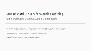
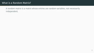
![1955: Random Symmetric Matrices
Eugene Wigner
Energy levels of heavy nuclei,
compared with the random
matrix theory prediction.
Source: [Rosenzweig and Porter,
1960]
4](https://image.slidesharecdn.com/randommatrixlearning-210710202533/85/Random-Matrix-Theory-and-Machine-Learning-Part-1-10-320.jpg)
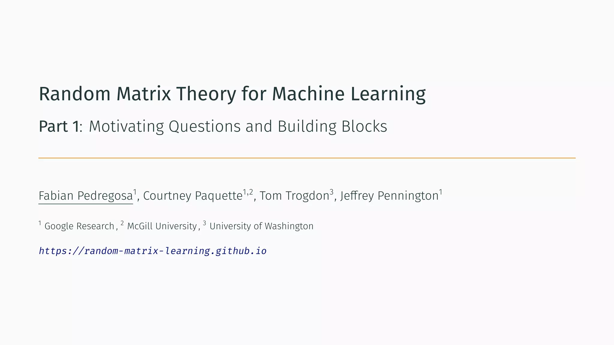
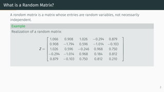
![Model for high-dimensional phenomena
• Number Theory [Montgomery, 1973,
Keating, 1993].
• Graph Theory [Erdos and Rényi, 1960].
• Finance [Bouchaud and Potters, 2009].
• Wireless communication [Tulino et al.,
2004]
• Machine Learning ... Distribution function of gaps between eigenvalues compared
with histogram of gaps between ζ zeros. Source: [Odlyzko, 1987]
5](https://image.slidesharecdn.com/randommatrixlearning-210710202533/85/Random-Matrix-Theory-and-Machine-Learning-Part-1-11-320.jpg)
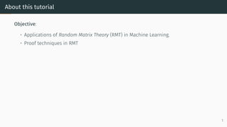
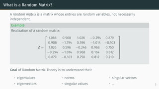
![Random Matrices in Machine Learning: Loss Landscape
Spin Glass model of the Loss Landscape
Early: [Amit et al., 1985, Gardner and Derrida, 1988, Dotsenko, 1995]
Late: [Dauphin et al., 2014, Sagun et al., 2014, Choromanska et al., 2015, Baity-Jesi et al., 2018]
Loss study through spin-glass model. Scaled test losses for the spin-glass (left) and the neural
network (right). Source: Choromanska et al. [2015] The Loss Surfaces of Multilayer Networks.
6](https://image.slidesharecdn.com/randommatrixlearning-210710202533/85/Random-Matrix-Theory-and-Machine-Learning-Part-1-12-320.jpg)
![Random Matrices in Machine Learning: Loss Landscape
New methods and software1,2,3
to compute
Hessian eigenvalues of large models
[Ghorbani et al., 2019, Yao et al., 2020,
Papyan, 2020]
1
https://github.com/amirgholami/PyHessian
2
https://github.com/google/spectral-density/
3
https://github.com/deep-lab/DeepnetHessian
Source: [Papyan, 2020]
7](https://image.slidesharecdn.com/randommatrixlearning-210710202533/85/Random-Matrix-Theory-and-Machine-Learning-Part-1-13-320.jpg)
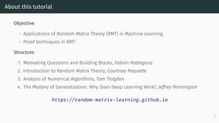
![Random Matrices in Machine Learning: Loss Landscape
New methods and software1,2,3
to compute
Hessian eigenvalues of large models
[Ghorbani et al., 2019, Yao et al., 2020,
Papyan, 2020]
1
https://github.com/amirgholami/PyHessian
2
https://github.com/google/spectral-density/
3
https://github.com/deep-lab/DeepnetHessian
RMT model for the Hessian still an open
problem [Liao and Mahoney, 2021,
Baskerville et al., 2021] ...
Source: [Papyan, 2020]
7](https://image.slidesharecdn.com/randommatrixlearning-210710202533/85/Random-Matrix-Theory-and-Machine-Learning-Part-1-14-320.jpg)
![Random Matrices in Machine Learning: Numerical Algorithms
Analyze algorithms with random data.
• Simplex [Borgwardt, 1987, Smale, 1983, Spielman
and Teng, 2004, Vershynin, 2009] etc.
• Conjugate Gradient [Deift and Trogdon, 2017,
Paquette and Trogdon, 2020]
• Acceleration [Pedregosa and Scieur, 2020,
Lacotte and Pilanci, 2020]
8](https://image.slidesharecdn.com/randommatrixlearning-210710202533/85/Random-Matrix-Theory-and-Machine-Learning-Part-1-15-320.jpg)
![Random Matrices in Machine Learning: Numerical Algorithms
Analyze algorithms with random data.
• Simplex [Borgwardt, 1987, Smale, 1983, Spielman
and Teng, 2004, Vershynin, 2009] etc.
• Conjugate Gradient [Deift and Trogdon, 2017,
Paquette and Trogdon, 2020]
• Acceleration [Pedregosa and Scieur, 2020,
Lacotte and Pilanci, 2020]
Topic of Part 3 of this tutorial
8](https://image.slidesharecdn.com/randommatrixlearning-210710202533/85/Random-Matrix-Theory-and-Machine-Learning-Part-1-16-320.jpg)
![Random Matrices in Machine Learning: Generalization
As a model for generalization [Hastie et al., 2019,
Mei and Montanari, 2019, Adlam and Pennington, 2020,
Liao et al., 2020]
Random Matrices can be used to model the double
descent generalization curve. Source: [Mei and Montanari,
2019] The generalization error of random features regression:
Precise asymptotics and double descent curve
9](https://image.slidesharecdn.com/randommatrixlearning-210710202533/85/Random-Matrix-Theory-and-Machine-Learning-Part-1-17-320.jpg)
![Random Matrices in Machine Learning: Generalization
As a model for generalization [Hastie et al., 2019,
Mei and Montanari, 2019, Adlam and Pennington, 2020,
Liao et al., 2020]
Random Matrices can be used to model the double
descent generalization curve. Source: [Mei and Montanari,
2019] The generalization error of random features regression:
Precise asymptotics and double descent curve
Part 4 of this tutorial 9](https://image.slidesharecdn.com/randommatrixlearning-210710202533/85/Random-Matrix-Theory-and-Machine-Learning-Part-1-18-320.jpg)

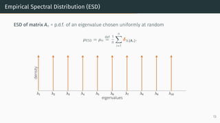
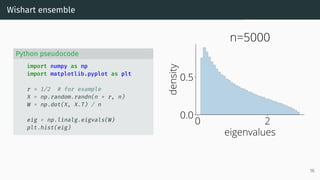
![Wigner Semicircle Law
µESD converges as n → ∞ to the semicircular distribution,
µSC(x)
def
=
1
2π
p
(4 − x2)+ dx .
2 0 2
eigenvalues
0.0
0.2
density
µSC
Wigner semicircle
To know more: [Tao, 2012, Bai and Silverstein, 2010].
14](https://image.slidesharecdn.com/randommatrixlearning-210710202533/85/Random-Matrix-Theory-and-Machine-Learning-Part-1-35-320.jpg)
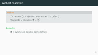

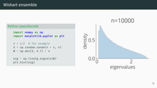
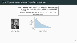
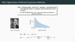
![Limit of Wishart matrices
Marchenko-Pastur (MP) law [Marčenko and Pastur, 1967]
As n, d → ∞, d
n → r, µESD converges to the Marchenko-Pastur distribution:
µMP(x)
def
= (1 − 1
r )+δ0(x)
| {z }
nonzero if r > 1
+
p
(λ+ − x)(x − λ−)
2πr x
1x∈[λ−,λ+] dx .
with λ−
= (1 −
√
r)2
, λ+
= (1 +
√
r)2
0 2
eigenvalues
0.0
0.5
density
Marchenko-Pastur
λ −
λ +
17](https://image.slidesharecdn.com/randommatrixlearning-210710202533/85/Random-Matrix-Theory-and-Machine-Learning-Part-1-46-320.jpg)
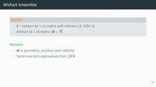
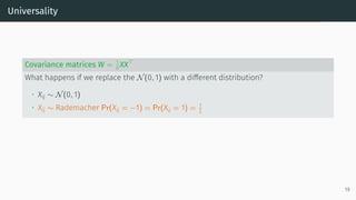
![The r = d
n
parameter
• r < 1 =⇒ d < n =⇒ W is product of two fat matrices.
• r > 1 =⇒ d > n =⇒ W is product of two thin matrices (rank-deficient).
1 2
eigenvalues
0.0
0.5
1.0
density
λ −
λ +
r=0.2
µMP(x)
def
= (1 − 1
r )+δ0(x)
| {z }
nonzero if r > 1
+
p
(λ+ − x)(x − λ−)
2πr x
1x∈[λ−,λ+] dx .
18](https://image.slidesharecdn.com/randommatrixlearning-210710202533/85/Random-Matrix-Theory-and-Machine-Learning-Part-1-47-320.jpg)
![The r = d
n
parameter
• r < 1 =⇒ d < n =⇒ W is product of two fat matrices.
• r > 1 =⇒ d > n =⇒ W is product of two thin matrices (rank-deficient).
0 2
eigenvalues
0.0
0.5
1.0
density
λ −
λ +
r=0.5
µMP(x)
def
= (1 − 1
r )+δ0(x)
| {z }
nonzero if r > 1
+
p
(λ+ − x)(x − λ−)
2πr x
1x∈[λ−,λ+] dx .
18](https://image.slidesharecdn.com/randommatrixlearning-210710202533/85/Random-Matrix-Theory-and-Machine-Learning-Part-1-48-320.jpg)
![The r = d
n
parameter
• r < 1 =⇒ d < n =⇒ W is product of two fat matrices.
• r > 1 =⇒ d > n =⇒ W is product of two thin matrices (rank-deficient).
0 2
eigenvalues
0
1
2
density
λ −
λ +
r=0.9
µMP(x)
def
= (1 − 1
r )+δ0(x)
| {z }
nonzero if r > 1
+
p
(λ+ − x)(x − λ−)
2πr x
1x∈[λ−,λ+] dx .
18](https://image.slidesharecdn.com/randommatrixlearning-210710202533/85/Random-Matrix-Theory-and-Machine-Learning-Part-1-49-320.jpg)
![The r = d
n
parameter
• r < 1 =⇒ d < n =⇒ W is product of two fat matrices.
• r > 1 =⇒ d > n =⇒ W is product of two thin matrices (rank-deficient).
0 2 4
eigenvalues
0
2
4
density
λ −
λ +
r=1.0
µMP(x)
def
= (1 − 1
r )+δ0(x)
| {z }
nonzero if r > 1
+
p
(λ+ − x)(x − λ−)
2πr x
1x∈[λ−,λ+] dx .
18](https://image.slidesharecdn.com/randommatrixlearning-210710202533/85/Random-Matrix-Theory-and-Machine-Learning-Part-1-50-320.jpg)
![The r = d
n
parameter
• r < 1 =⇒ d < n =⇒ W is product of two fat matrices.
• r > 1 =⇒ d > n =⇒ W is product of two thin matrices (rank-deficient).
0.0 2.5 5.0
eigenvalues
0.0
0.1
0.2
0.3
density
λ −
λ +
r=2.0
µMP(x)
def
= (1 − 1
r )+δ0(x)
| {z }
nonzero if r > 1
+
p
(λ+ − x)(x − λ−)
2πr x
1x∈[λ−,λ+] dx .
18](https://image.slidesharecdn.com/randommatrixlearning-210710202533/85/Random-Matrix-Theory-and-Machine-Learning-Part-1-51-320.jpg)
![The r = d
n
parameter
• r < 1 =⇒ d < n =⇒ W is product of two fat matrices.
• r > 1 =⇒ d > n =⇒ W is product of two thin matrices (rank-deficient).
0 5 10
eigenvalues
0.00
0.05
0.10
density
λ −
λ +
r=5.0
µMP(x)
def
= (1 − 1
r )+δ0(x)
| {z }
nonzero if r > 1
+
p
(λ+ − x)(x − λ−)
2πr x
1x∈[λ−,λ+] dx .
18](https://image.slidesharecdn.com/randommatrixlearning-210710202533/85/Random-Matrix-Theory-and-Machine-Learning-Part-1-52-320.jpg)
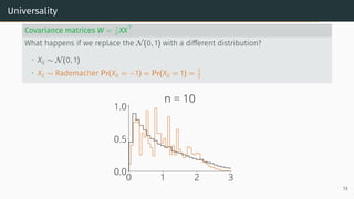


![Universality
Universality
• Statistics only mildly depend on the lower order moments of distribution of the
entries
Example: Marchenko-Pastur [Marčenko and Pastur, 1967]
Let X be a d × n random matrix with i.i.d. entries that verifies
E[Xij] = 0, E[X2
ij] = 1, E[X4
ij] < ∞
Universality: As n, d → ∞ with d
n → r, the ESD of W = XXT
n converges to
Marchenko-Pastur(r)
20](https://image.slidesharecdn.com/randommatrixlearning-210710202533/85/Random-Matrix-Theory-and-Machine-Learning-Part-1-60-320.jpg)
![May others ...
Other matrix ensembles
• Ginibre. Let Gn be n × n matrix of i.i.d. N(0, 1), (bilinear games [Domingo-Enrich et al., 2020])
(Circle law) ESD of Gn/
√
n → Unif(disk) .
• Uniform probability measure on orthogonal matrices. V ∼ Unif(O(n)),
ESD of V → Unif(S1
) .
21](https://image.slidesharecdn.com/randommatrixlearning-210710202533/85/Random-Matrix-Theory-and-Machine-Learning-Part-1-61-320.jpg)


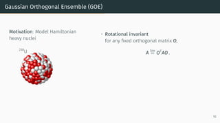
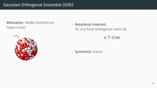
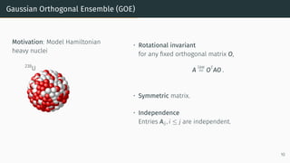
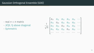
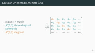
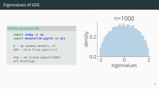
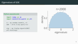
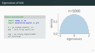
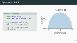
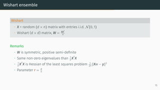
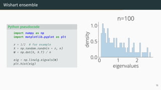
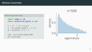
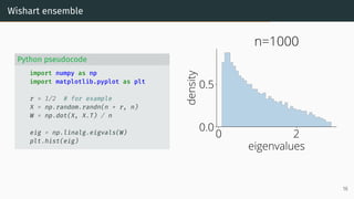
This document provides an introduction to random matrix theory and its applications in machine learning. It discusses several classical random matrix ensembles like the Gaussian Orthogonal Ensemble (GOE) and Wishart ensemble. These ensembles are used to model phenomena in fields like number theory, physics, and machine learning. Specifically, the GOE is used to model Hamiltonians of heavy nuclei, while the Wishart ensemble relates to the Hessian of least squares problems. The tutorial will cover applications of random matrix theory to analyzing loss landscapes, numerical algorithms, and the generalization properties of machine learning models.


![谷歌留痕技术 [ 𝙩𝙤𝙥 𝟮𝟯𝟯. 𝙘 𝙤𝙢 ]](https://cdn.slidesharecdn.com/ss_thumbnails/top233-260130174328-3833018c-thumbnail.jpg?width=640&height=640&fit=bounds)