Download as PDF, PPTX


![. . . . . .
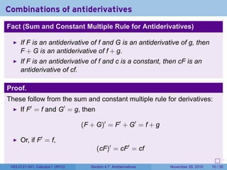
Why the MVT is the MITC
Most Important Theorem In Calculus!
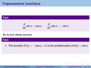
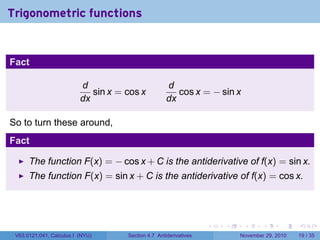
Theorem
Let f′
= 0 on an interval (a, b). Then f is constant on (a, b).
Proof.
Pick any points x and y in (a, b) with x y. Then f is continuous on
[x, y] and differentiable on (x, y). By MVT there exists a point z in (x, y)
such that
f(y) − f(x)
y − x
= f′
(z) =⇒ f(y) = f(x) + f′
(z)(y − x)
But f′
(z) = 0, so f(y) = f(x). Since this is true for all x and y in (a, b),
then f is constant.
V63.0121.041, Calculus I (NYU) Section 4.7 Antiderivatives November 29, 2010 7 / 35](https://image.slidesharecdn.com/lesson23-antiderivatives041slides-101129215246-phpapp01/85/Lesson-23-Antiderivatives-Section-041-slides-13-320.jpg)


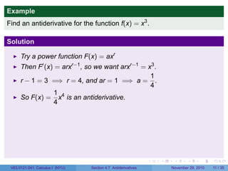
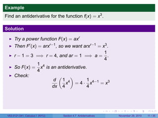
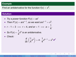
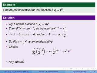
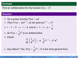
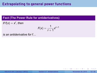
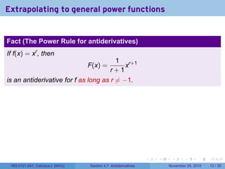
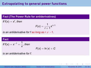


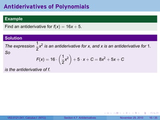
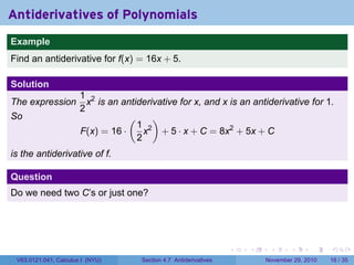
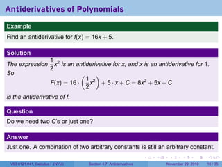


The document covers the concept of antiderivatives as part of a Calculus I course at New York University, detailing methods to find functions whose derivatives yield specified elementary functions. It includes explanations of topics such as power functions, combinations, and applying the power rule for antiderivatives, along with examples for practice. Additionally, it emphasizes the importance of the Mean Value Theorem and provides theorems regarding functions with the same derivatives.