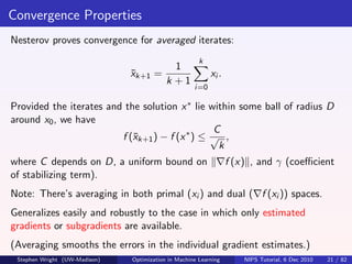
The document summarizes optimization algorithms for machine learning applications. It discusses first-order methods like gradient descent, accelerated methods like Nesterov's algorithm, and non-monotone methods like Barzilai-Borwein. Gradient descent converges at a rate of 1/k, while methods like heavy-ball, conjugate gradient, and Nesterov's algorithm can achieve faster linear or 1/k^2 convergence rates depending on the problem structure. The document provides convergence analysis and rate results for various first-order optimization algorithms applied to machine learning problems.

![Exact minimizing αk : Faster rate?
Take αk to be the exact minimizer of f along − f (xk ). Does this yield a
better rate of linear convergence?
Consider the convex quadratic f (x) = (1/2)x T Ax. (Thus x ∗ = 0 and
f (x ∗ ) = 0.) Here κ is the condition number of A.
We have f (xk ) = Axk . Exact minimizing αk :
xk A2 xk
T
1
αk = T A3 x
= arg min (xk − αAxk )T A(xk − αAxk ),
xk k α 2
1 1
which is in the interval L, µ . Can show that
2k
∗ 2
f (xk ) − f (x ) ≤ 1− [f (x0 ) − f (x ∗ )].
κ+1
No improvement in the linear rate over constant steplength.
Stephen Wright (UW-Madison) Optimization in Machine Learning NIPS Tutorial, 6 Dec 2010 9 / 82](https://image.slidesharecdn.com/sjw-nips10-110512225703-phpapp01/85/NIPS2010-optimization-algorithms-in-machine-learning-9-320.jpg)
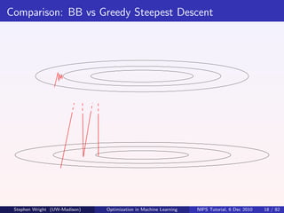
![A Non-Monotone Gradient Method: Barzilai-Borwein
(Barzilai & Borwein 1988) BB is a gradient method, but with an unusual
choice of αk . Allows f to increase (sometimes dramatically) on some steps.
2
xk+1 = xk − αk f (xk ), αk := arg min sk − αzk ,
α
where
sk := xk − xk−1 , zk := f (xk ) − f (xk−1 ).
Explicitly, we have
T
sk zk
αk = T
.
zk zk
Note that for convex quadratic f = (1/2)x T Ax, we have
T
sk Ask
αk = T
∈ [L−1 , µ−1 ].
sk A2 sk
Hence, can view BB as a kind of quasi-Newton method, with the Hessian
−1
approximated by αk I .
Stephen Wright (UW-Madison) Optimization in Machine Learning NIPS Tutorial, 6 Dec 2010 17 / 82](https://image.slidesharecdn.com/sjw-nips10-110512225703-phpapp01/85/NIPS2010-optimization-algorithms-in-machine-learning-17-320.jpg)
![Primal-Dual Averaging
(see Nesterov 2009) Basic step:
k
1 γ
xk+1 = arg min [f (xi ) + f (xi )T (x − xi )] + √ x − x0 2
x k +1 k
i=0
γ
= arg min ¯T
gk x + √ x − x0 2 ,
x k
k
where gk :=
¯ i=0 f (xi )/(k + 1) — the averaged gradient.
The last term is always centered at the first iterate x0 .
Gradient information is averaged over all steps, with equal weights.
γ is constant - results can be sensitive to this value.
The approach still works for convex nondifferentiable f , where f (xi )
is replaced by a vector from the subgradient ∂f (xi ).
Stephen Wright (UW-Madison) Optimization in Machine Learning NIPS Tutorial, 6 Dec 2010 20 / 82](https://image.slidesharecdn.com/sjw-nips10-110512225703-phpapp01/85/NIPS2010-optimization-algorithms-in-machine-learning-20-320.jpg)
![Example: Nesterov’s Constant Step Scheme for minx∈Ω f (x). Requires
just only calculation to be changed from the unconstrained version.
0: Choose x0 , α0 ∈ (0, 1); set y0 ← x0 , q ← 1/κ = µ/L.
1 1
k: xk+1 ← arg miny ∈Ω 2 y − [yk − L f (yk )] 2 ;
2
2 2
solve for αk+1 ∈ (0, 1): αk+1 = (1 − αk+1 )αk + qαk+1 ;
2
set βk = αk (1 − αk )/(αk + αk+1 );
set yk+1 ← xk+1 + βk (xk+1 − xk ).
Convergence theory is unchanged.
Stephen Wright (UW-Madison) Optimization in Machine Learning NIPS Tutorial, 6 Dec 2010 23 / 82](https://image.slidesharecdn.com/sjw-nips10-110512225703-phpapp01/85/NIPS2010-optimization-algorithms-in-machine-learning-23-320.jpg)

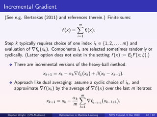
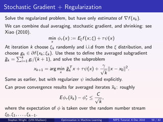
![“Classical” Stochastic Approximation
Denote by G (x, ξ) ths subgradient estimate generated at x. For
unbiasedness need Eξ G (x, ξ) ∈ ∂f (x).
Basic SA Scheme: At iteration k, choose ξk i.i.d. according to distribution
P, choose some αk > 0, and set
xk+1 = xk − αk G (xk , ξk ).
Note that xk+1 depends on all random variables up to iteration k, i.e.
ξ[k] := {ξ1 , ξ2 , . . . , ξk }.
When f is strongly convex, the analysis of convergence of E ( xk − x ∗ 2 ) is
fairly elementary - see Nemirovski et al (2009).
Stephen Wright (UW-Madison) Optimization in Machine Learning NIPS Tutorial, 6 Dec 2010 30 / 82](https://image.slidesharecdn.com/sjw-nips10-110512225703-phpapp01/85/NIPS2010-optimization-algorithms-in-machine-learning-30-320.jpg)
![Rate: 1/k
Define ak = 1 E ( xk − x ∗ 2 ). Assume there is M > 0 such that
2
E ( G (x, ξ) 2 ) ≤ M 2 for all x of interest. Thus
1
xk+1 − x ∗ 2
2
2
1
= xk − αk G (xk , ξk ) − x ∗ 2
2
1 1 2
= xk − x ∗ 2 − αk (xk − x ∗ )T G (xk , ξk ) + αk G (xk , ξk ) 2 .
2
2 2
Taking expectations, get
1 2
ak+1 ≤ ak − αk E [(xk − x ∗ )T G (xk , ξk )] + αk M 2 .
2
For middle term, have
E [(xk − x ∗ )T G (xk , ξk )] = Eξ[k−1] Eξk [(xk − x ∗ )T G (xk , ξk )|ξ[k−1] ]
= Eξ[k−1] (xk − x ∗ )T gk ,
Stephen Wright (UW-Madison) Optimization in Machine Learning NIPS Tutorial, 6 Dec 2010 31 / 82](https://image.slidesharecdn.com/sjw-nips10-110512225703-phpapp01/85/NIPS2010-optimization-algorithms-in-machine-learning-31-320.jpg)
![... where
gk := Eξk [G (xk , ξk )|ξ[k−1] ] ∈ ∂f (xk ).
By strong convexity, have
1
(xk − x ∗ )T gk ≥ f (xk ) − f (x ∗ ) + µ xk − x ∗ 2
≥ µ xk − x ∗ 2 .
2
Hence by taking expectations, we get E [(xk − x ∗ )T gk ] ≥ 2µak . Then,
substituting above, we obtain
1 2
ak+1 ≤ (1 − 2µαk )ak + αk M 2
2
When
1
αk ≡ ,
kµ
a neat inductive argument (exercise!) reveals the 1/k rate:
Q M2
ak ≤ , for Q := max x1 − x ∗ 2 , .
2k µ2
Stephen Wright (UW-Madison) Optimization in Machine Learning NIPS Tutorial, 6 Dec 2010 32 / 82](https://image.slidesharecdn.com/sjw-nips10-110512225703-phpapp01/85/NIPS2010-optimization-algorithms-in-machine-learning-32-320.jpg)
![Analysis of Robust SA
The analysis is again elementary. As above (using i instead of k), have:
1
αi E [(xi − x ∗ )T gi ] ≤ ai − ai+1 + αi2 M 2 .
2
By convexity of f , and gi ∈ ∂f (xi ):
f (x ∗ ) ≥ f (xi ) + giT (x ∗ − xi ),
thus
1
αi E [f (xi ) − f (x ∗ )] ≤ ai − ai+1 + αi2 M 2 ,
2
so by summing iterates i = 1, 2, . . . , k, telescoping, and using ak+1 > 0:
k k
1
αi E [f (xi ) − f (x ∗ )] ≤ a1 + M 2 αi2 .
2
i=1 i=1
Stephen Wright (UW-Madison) Optimization in Machine Learning NIPS Tutorial, 6 Dec 2010 35 / 82](https://image.slidesharecdn.com/sjw-nips10-110512225703-phpapp01/85/NIPS2010-optimization-algorithms-in-machine-learning-35-320.jpg)
![Thus dividing by i=1 αi :
k k
i=1 αi f (xi ) a1 + 1 M 2 2
i=1 αi
E k
− f (x ∗ ) ≤ 2
k
.
i=1 αi i=1 αi
By convexity, we have
k
i=1 αi f (xi )
f (¯k ) ≤
x k
,
i=1 αi
so obtain the fundamental bound:
1 k
a1 + 2 M 2 2
i=1 αi
E [f (¯k ) − f (x ∗ )] ≤
x k
.
i=1 αi
Stephen Wright (UW-Madison) Optimization in Machine Learning NIPS Tutorial, 6 Dec 2010 36 / 82](https://image.slidesharecdn.com/sjw-nips10-110512225703-phpapp01/85/NIPS2010-optimization-algorithms-in-machine-learning-36-320.jpg)
![θ
By substituting αi = √ ,
M i
we obtain
1 k 1
a1 + 2 θ2
E [f (¯k ) − f (x ∗ )] ≤
x θ k
i=1 i
1
√
M i=1 i
a1 + θ2 log(k + 1)
≤ θ
√
M k
a1
=M + θ log(k + 1) k −1/2 .
θ
That’s it!
Other variants: constant stepsizes αk for a fixed “budget” of iterations;
periodic restarting; averaging just over the recent iterates. All can be
analyzed with the basic bound above.
Stephen Wright (UW-Madison) Optimization in Machine Learning NIPS Tutorial, 6 Dec 2010 37 / 82](https://image.slidesharecdn.com/sjw-nips10-110512225703-phpapp01/85/NIPS2010-optimization-algorithms-in-machine-learning-37-320.jpg)
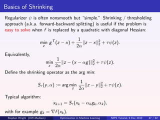
![“Practical” Instances of ψ
Cases for which the subproblem is simple:
ψ(z) = z 1 . Thus Sτ (y , α) = sign(y ) max(|y | − ατ, 0). When y
complex, have
max(|y | − τ α, 0)
Sτ (y , α) = y.
max(|y | − τ α, 0) + τ α
ψ(z) = g ∈G z[g ] 2 or ψ(z) = g ∈G z[g ] ∞, where z[g ] , g ∈ G
are non-overlapping subvectors of z. Here
max(|y[g ] | − τ α, 0)
Sτ (y , α)[g ] = y .
max(|y[g ] | − τ α, 0) + τ α [g ]
Stephen Wright (UW-Madison) Optimization in Machine Learning NIPS Tutorial, 6 Dec 2010 48 / 82](https://image.slidesharecdn.com/sjw-nips10-110512225703-phpapp01/85/NIPS2010-optimization-algorithms-in-machine-learning-48-320.jpg)
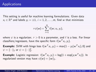
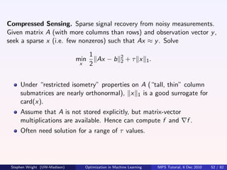
![Applications
LASSO for variable selection. Originally stated as
1
Ax − b 2 such that x 1 ≤ T ,
min 2
2 x
for parameter T > 0. Equivalent to an “ 2 - 1 ” formulation:
1 2
min Ax − b 2 +τ x 1, for some τ > 0.
x 2
Group LASSO for selection of variable “groups.”
1 2
min Ax − b 2 + x[g ] 2 ,
x 2
g ∈G
with each [g ] a subset of indices {1, 2, . . . , n}.
When groups [g ] are disjoint, easy to solve the subproblem.
Still true if · 2 is replaced by · ∞ .
When groups overlap, can replicate variables, to have one copy of
each variable in each group — thus reformulate as non-overlapping.
Stephen Wright (UW-Madison) Optimization in Machine Learning NIPS Tutorial, 6 Dec 2010 51 / 82](https://image.slidesharecdn.com/sjw-nips10-110512225703-phpapp01/85/NIPS2010-optimization-algorithms-in-machine-learning-51-320.jpg)

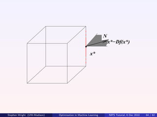
![For a polyhedral Ω, the active manifold is the face on which x ∗ lies.
Example: For Ω = [0, 1]n , active manifold consists of z with
= 1
if xi∗ = 1
zi = 0 if xi∗ = 0
∈ [0, 1] if xi∗ ∈ (0, 1).
M
x*
Can parametrize M with a single variable.
Stephen Wright (UW-Madison) Optimization in Machine Learning NIPS Tutorial, 6 Dec 2010 62 / 82](https://image.slidesharecdn.com/sjw-nips10-110512225703-phpapp01/85/NIPS2010-optimization-algorithms-in-machine-learning-62-320.jpg)
![How Might This Help?
Consider again logistic regression with regularizer ψ(w ) = w 1 .
m
1 T
L(w ) = − w T xi − log(1 + e w xi ) .
m
yi =−1 i=1
Requires calculation of Xw where X = [xiT ]m . (Can be cheap if w has
i=1
few nonzeros.) For gradient, have
T
1 −(1 + e w xi )−1 , yi = −1,
L(w ) = X T u, where ui = T
m (1 + e −w xi )−1 , yi = +1.
requires m exponentials, and a matrix-vector multiply by X (with a full
vector u).
If just a subset G of components needed, multiply by a column submatrix
T
X·G — much cheaper than full gradient if |G| n.
Stephen Wright (UW-Madison) Optimization in Machine Learning NIPS Tutorial, 6 Dec 2010 66 / 82](https://image.slidesharecdn.com/sjw-nips10-110512225703-phpapp01/85/NIPS2010-optimization-algorithms-in-machine-learning-66-320.jpg)
![Constraints and Regularizers Complicate Things
For minx∈Ω f (x), need to put enough components into Gk to stay feasible,
as well as make progress.
Example: min f (x1 , x2 ) with x1 + x2 = 1. Relaxation with Gk = {1} or
Gk = {2} won’t work.
For separable regularizer (e.g. Group LASSO) with
ψ(x) = ψg (x[g ] ),
g ∈G
need to ensure that Gk is a union of the some index subsets [g ]. i.e. the
relaxation components must be consonant with the partitioning.
Stephen Wright (UW-Madison) Optimization in Machine Learning NIPS Tutorial, 6 Dec 2010 76 / 82](https://image.slidesharecdn.com/sjw-nips10-110512225703-phpapp01/85/NIPS2010-optimization-algorithms-in-machine-learning-76-320.jpg)
![Stochastic Coordinate Descent
Analysis tools of stochastic gradient may be useful. If steps have the form
xk+1 = xk − αk gk , where
[ f (xk )]i if i ∈ Gk
gk (i) =
0 otherwise,
With suitable random selection of Gk can ensure that gk (appropriately
scaled) is an unbiased estimate of f (xk ). Hence can apply SGD
techniqes discussed earlier, to choose αk and obtain convergence.
Nesterov (2010) proposes another randomized approach for the
unconstrained problem with known separate Lipschitz constants Li :
∂fi ∂fi
(x + hei ) − (x) ≤ Li |h|, i = 1, 2, . . . , n.
∂xi ∂xi
(Works with blocks too, instead of individual components.)
Stephen Wright (UW-Madison) Optimization in Machine Learning NIPS Tutorial, 6 Dec 2010 79 / 82](https://image.slidesharecdn.com/sjw-nips10-110512225703-phpapp01/85/NIPS2010-optimization-algorithms-in-machine-learning-79-320.jpg)
![At step k:
n
Choose index ik ∈ {1, 2, . . . , n} with probability pi := Li /( j=1 Lj );
Take gradient step in ik component:
1 ∂f
xk+1 = xk − ei .
Lik ∂xik k
Basic convergence result:
C
E [f (xk )] − f ∗ ≤ .
k
As for SA (earlier) but without any strong convexity assumption.
Can also get linear convergence results (in expectation) by assuming
strong convexity in f , according to different norms.
Can also accelerate in the usual fashion (see above), to improve expected
convergence rate to O(1/k 2 ).
Stephen Wright (UW-Madison) Optimization in Machine Learning NIPS Tutorial, 6 Dec 2010 80 / 82](https://image.slidesharecdn.com/sjw-nips10-110512225703-phpapp01/85/NIPS2010-optimization-algorithms-in-machine-learning-80-320.jpg)