Download as PDF, PPTX


![Method 1: Stieltjes transform
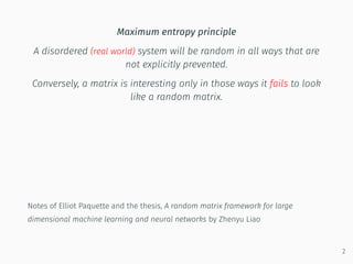
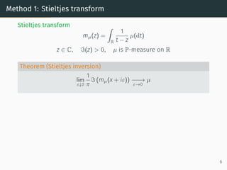
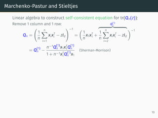
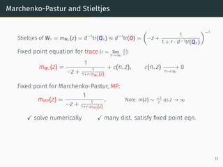
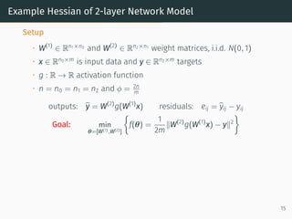
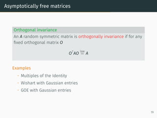
Stieltjes transform
mµ(z) =
Z
R
1
t − z
µ(dt)
z ∈ C, ℑ(z) > 0, µ is P-measure on R
Theorem (Stieltjes inversion)
lim
ε↓0
1
π
ℑ (mµ(x + iε)) −
−
−
→
ε→0
µ
Example: µ is law of Unif([−1, 1])
Stieltjes transform:
mµ(z) =
1
2
Z
R
1
t − z
1 ({|t| ≤ 1}) dt =
1
2
Z 1
−1
dt
t − z
=
1
2
log
1 − z
−1 − z
Inversion lim
ε↓0
ℑ
π
1
2
log
1 − z
−1 − z](https://image.slidesharecdn.com/randommatrixlearning1-210710203915/85/Random-Matrix-Theory-and-Machine-Learning-Part-2-10-320.jpg)
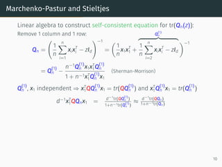
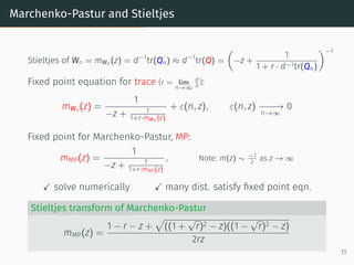


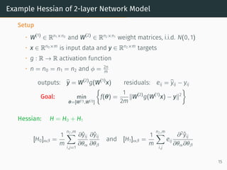
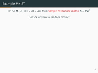
![Sample covariance matrices
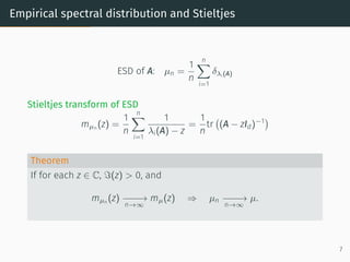
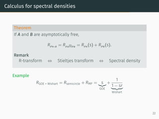
Set-up
• Covariance matrix, C, (symmetric, positive semi-definite matrix)
• Noise matrix, Z ∈ Rd×n
(mean 0, variance 1, i.i.d.)
• n1/δ
≤ d ≤ nδ
for some δ 0
• X = C1/2
Z; Form
XXT
n
• ∥C∥2 ≤ constant, independent of n
Theorem (Bai, Krishnaiah, Silverstein, Yin, ’80s-’90s)
Stieltjes of XXT
n = tr
Id − zXXT
n
−1
≈ n
d
e
m(z) +
1− d
n
d
n z
where e
m(z) = −z + 1
n tr[C(Id − e
m(z)C)−1
]
−1
✓ e
m(z) ≈ Stieltjes transform XT
X
n
✓ implicit eqn, solved numerically
13](https://image.slidesharecdn.com/randommatrixlearning1-210710203915/85/Random-Matrix-Theory-and-Machine-Learning-Part-2-28-320.jpg)
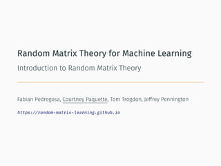
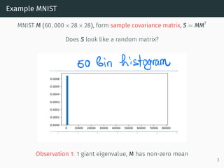
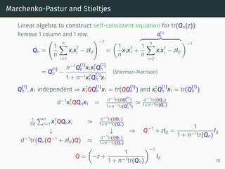
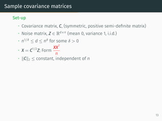
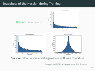
![Example Hessian of 2-layer Network Model
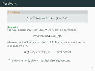
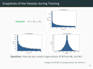
Setup
• W(1)
∈ Rn1×n0
and W(2)
∈ Rn2×n1
weight matrices, i.i.d. N(0, 1)
• x ∈ Rn0×m
is input data and y ∈ Rn2×m
targets
• g : R → R activation function
• n = n0 = n1 = n2 and ϕ = 2n
m
outputs: b
y = W(2)
g(W(1)
x) residuals: eij = b
yij − yij
Goal: min
θ=[W(1),W(2)]
f(θ) =
1
2m
∥W(2)
g(W(1)
x) − y∥2
15](https://image.slidesharecdn.com/randommatrixlearning1-210710203915/85/Random-Matrix-Theory-and-Machine-Learning-Part-2-31-320.jpg)
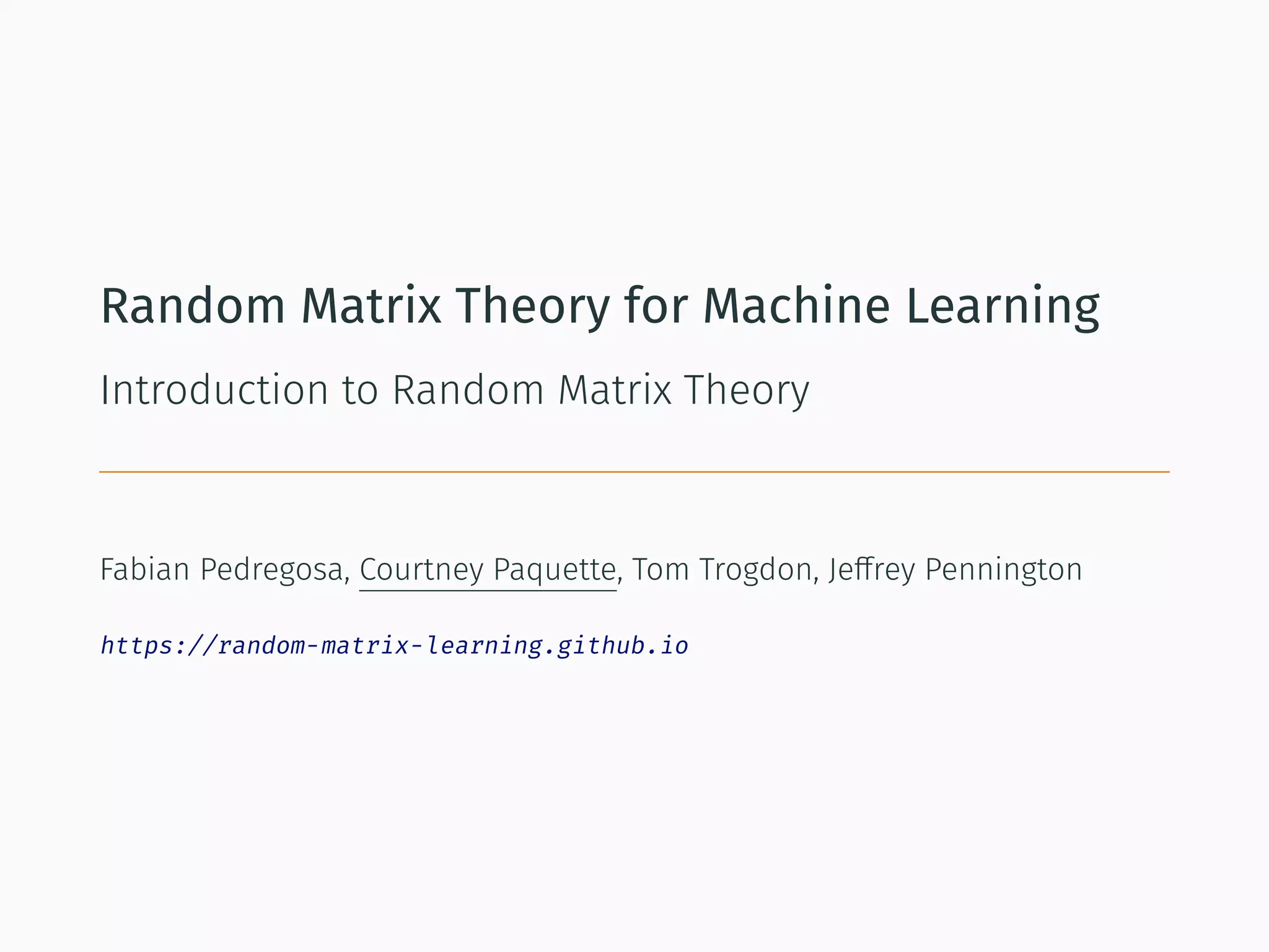
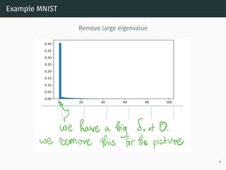
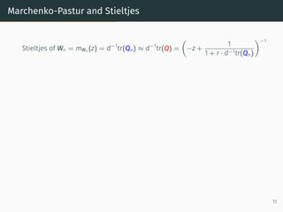
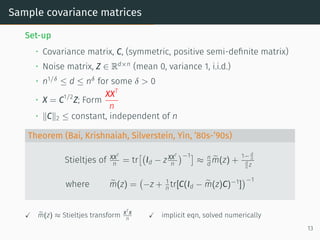
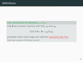
![Example Hessian of 2-layer Network Model
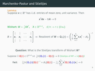
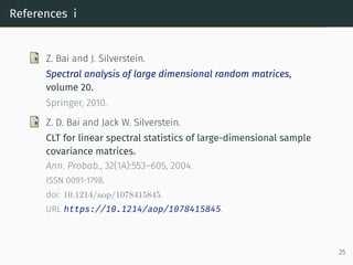
Setup
• W(1)
∈ Rn1×n0
and W(2)
∈ Rn2×n1
weight matrices, i.i.d. N(0, 1)
• x ∈ Rn0×m
is input data and y ∈ Rn2×m
targets
• g : R → R activation function
• n = n0 = n1 = n2 and ϕ = 2n
m
outputs: b
y = W(2)
g(W(1)
x) residuals: eij = b
yij − yij
Goal: min
θ=[W(1),W(2)]
f(θ) =
1
2m
∥W(2)
g(W(1)
x) − y∥2
Hessian: H = H0 + H1
[H0]αβ =
1
m
n2,m
X
i,j=1
∂ŷij
∂θα
∂ŷij
∂θβ
and [H1]αβ =
1
m
n2,m
X
i,j
eij
∂2
ŷij
∂θα∂θβ
15](https://image.slidesharecdn.com/randommatrixlearning1-210710203915/85/Random-Matrix-Theory-and-Machine-Learning-Part-2-32-320.jpg)


This document discusses the application of random matrix theory to machine learning, detailing concepts such as the Stieltjes transform, the r-transform, and their relevance to understanding sample covariance matrices and eigenvalues in neural networks. It includes specific examples leveraging the MNIST dataset to illustrate how these theories can be utilized to analyze data and simplify complex structures. Key insights involve the behavior of eigenvalues and the relationship between matrix randomness and neural network training dynamics.