Download as PDF, PPTX
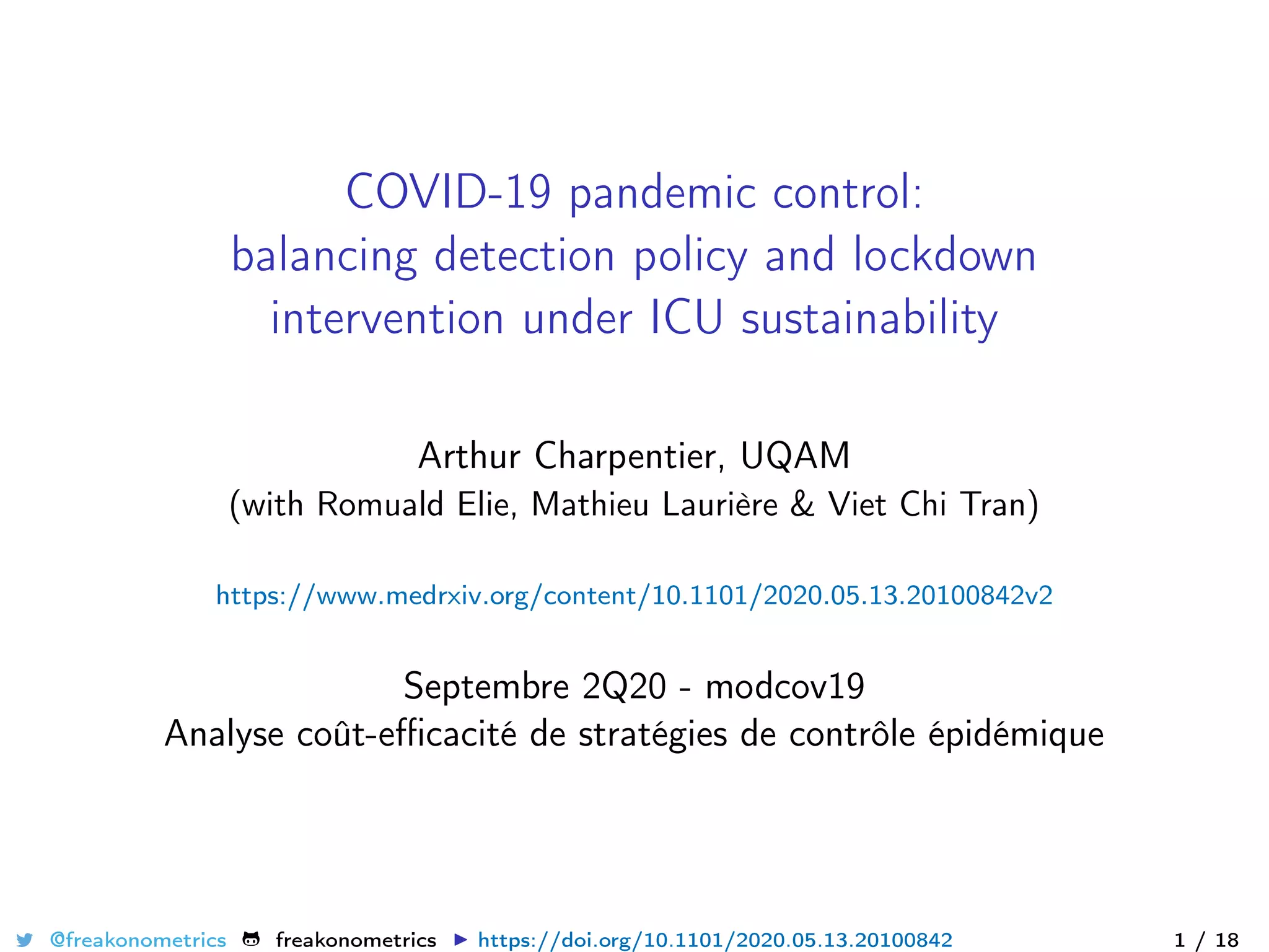

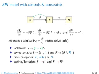
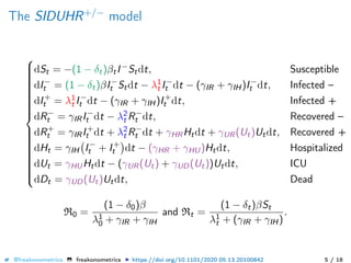
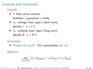
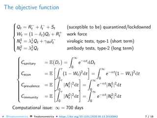
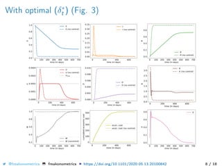
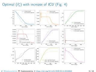
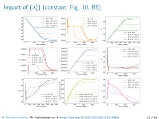
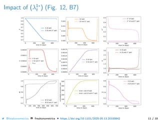
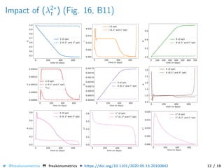

The document provides a mathematical model for controlling the COVID-19 pandemic by balancing detection policies and lockdown interventions to ensure the sustainability of ICU capacity. It discusses various strategies, including virological and antibody testing, and their impact on disease spread and healthcare resources. The objective is to minimize a composite cost function that considers public health and economic factors over time.


