The document summarizes a seminar presentation on Gaussian processes and their applications in machine learning. It introduces Gaussian processes, prior and posterior distributions, and how Gaussian processes can be used for regression and classification problems. It also discusses covariance functions and highlights areas of current research such as fast approximation algorithms and non-Gaussian likelihoods. Gaussian processes provide a flexible modeling approach that has outperformed traditional methods in applications like positioning systems and multi-user detection.

1. Gaussian Processes: Applications in Machine
Learning
Abhishek Agarwal
(05329022)
Under the Guidance of Prof. Sunita Sarawagi
KReSIT, IIT Bombay
Seminar Presentation
March 29, 2006
Abhishek Agarwal (05329022) Gaussian Processes: Applications in Machine Learning

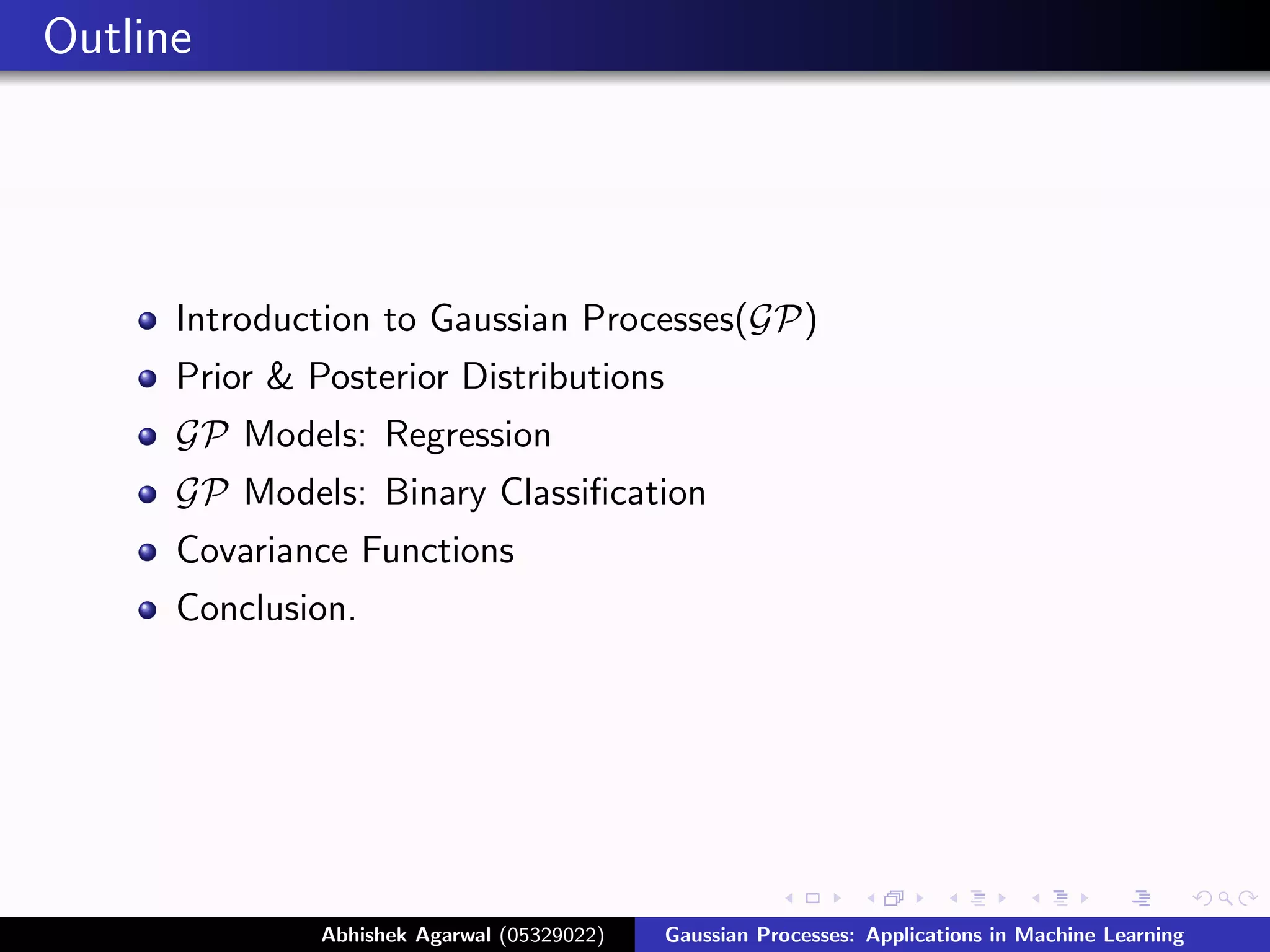
2. Outline
Introduction to Gaussian Processes(GP)
Prior & Posterior Distributions
GP Models: Regression
GP Models: Binary Classification
Covariance Functions
Conclusion.
Abhishek Agarwal (05329022) Gaussian Processes: Applications in Machine Learning

3. Introduction
Supervised Learning
Gaussian Processes
Defines distribution over functions.
Collection of random variables, any finite number of which
have joint Gaussian distributions.[1] [2]
f ∼ GP(m, k)
Hyperparameters and Covariance function.
Predictions
Abhishek Agarwal (05329022) Gaussian Processes: Applications in Machine Learning

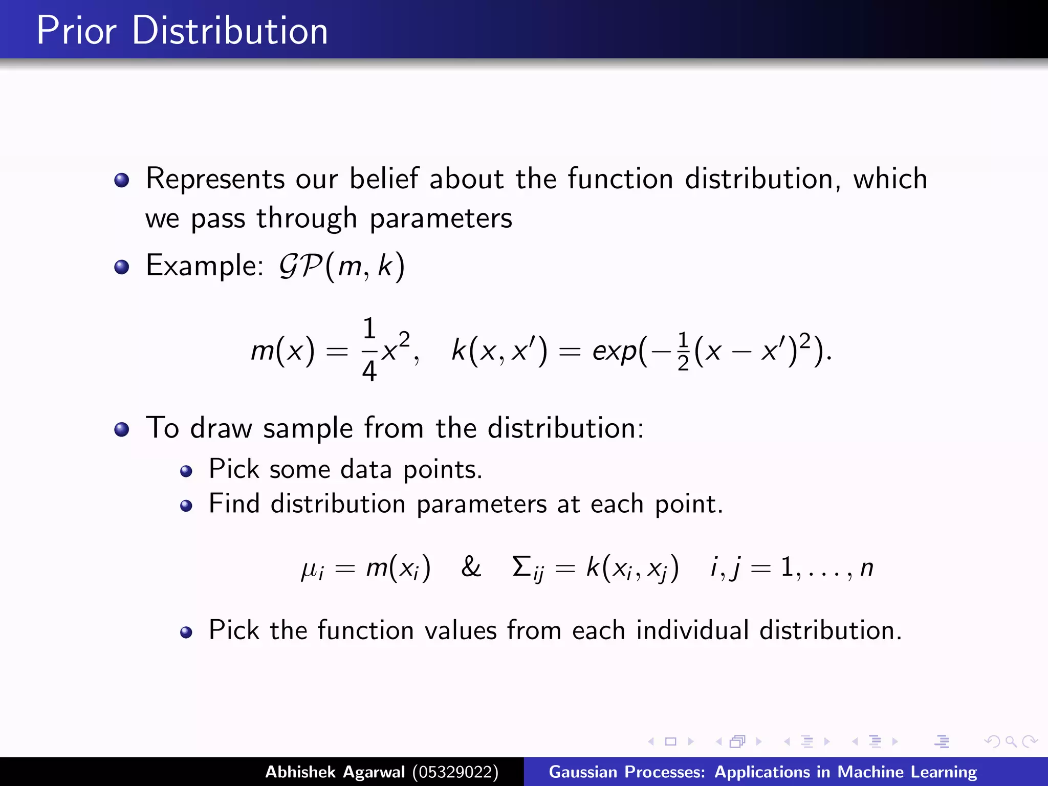
4. Prior Distribution
Represents our belief about the function distribution, which
we pass through parameters
Example: GP(m, k)
1
m(x) = x 2 , k(x, x ) = exp(− 1 (x − x )2 ).
2
4
To draw sample from the distribution:
Pick some data points.
Find distribution parameters at each point.
µi = m(xi ) & Σij = k(xi , xj ) i, j = 1, . . . , n
Pick the function values from each individual distribution.
Abhishek Agarwal (05329022) Gaussian Processes: Applications in Machine Learning

5. Prior Distribution(contd.)
9
8
7
6
function values
5
4
3
2
1
−5 −4 −3 −2 −1 0 1 2 3 4 5
data points
Figure: Prior distribution over function using Gaussian Process
Abhishek Agarwal (05329022) Gaussian Processes: Applications in Machine Learning

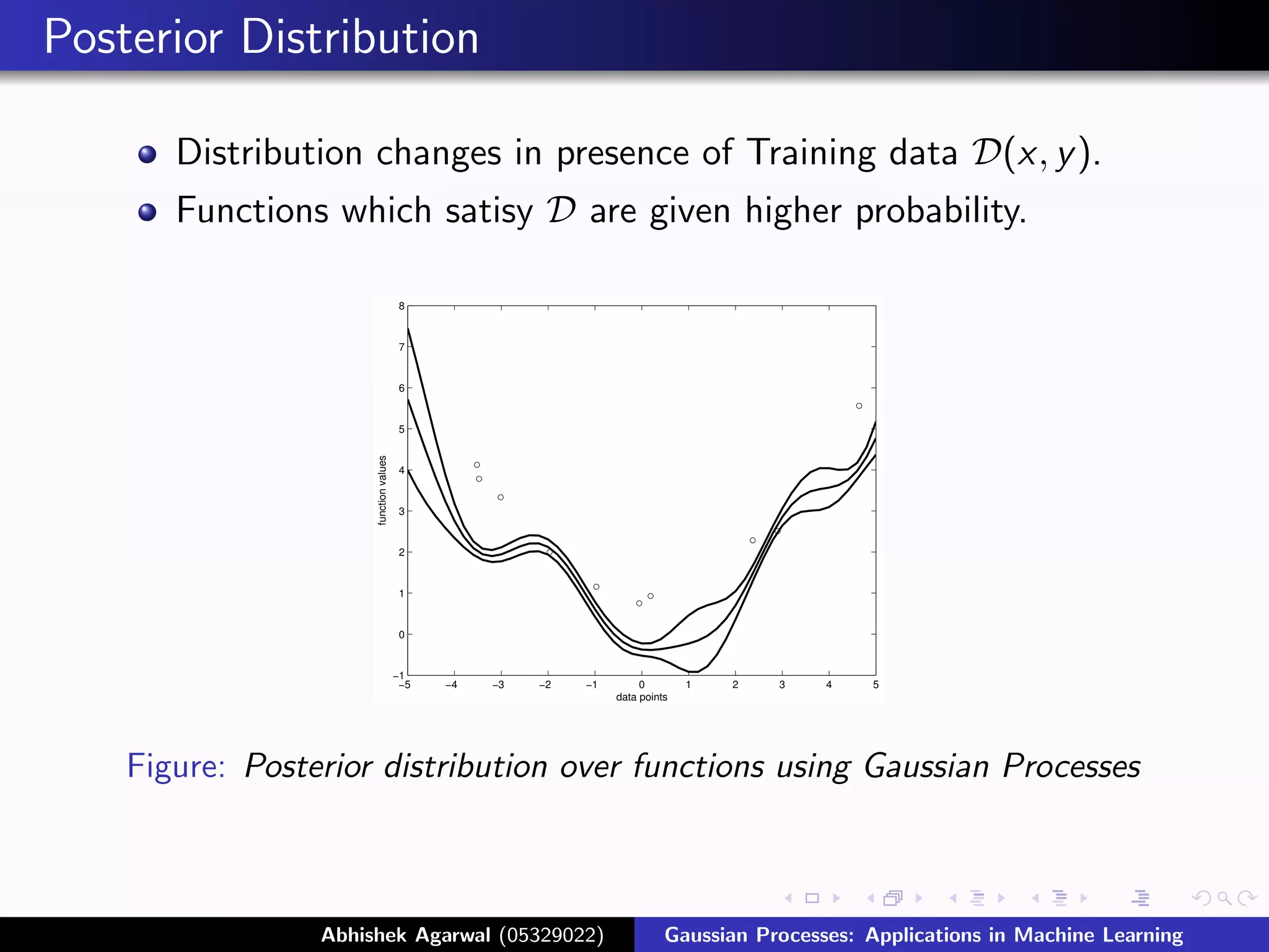
6. Posterior Distribution
Distribution changes in presence of Training data D(x, y ).
Functions which satisy D are given higher probability.
8
7
6
5
function values
4
3
2
1
0
−1
−5 −4 −3 −2 −1 0 1 2 3 4 5
data points
Figure: Posterior distribution over functions using Gaussian Processes
Abhishek Agarwal (05329022) Gaussian Processes: Applications in Machine Learning

7. Posterior Distribution (contd.)
Prediction for unlabeled data x∗
GP outputs the function distribution at x∗
Let f be the distribution at data points in D and f∗ at x∗
f and f∗ will have a joint Gaussian distribution, represented as:
f µ Σ Σ∗
∼
f∗ µ∗ Σ∗ T Σ∗∗
Conditional distribution of f∗ given f can be expressed as:
f∗ |f ∼ N ( µ∗ + Σ∗ T Σ−1 (f − µ), Σ∗∗ − Σ∗ T Σ−1 Σ∗ ) (1)
Abhishek Agarwal (05329022) Gaussian Processes: Applications in Machine Learning

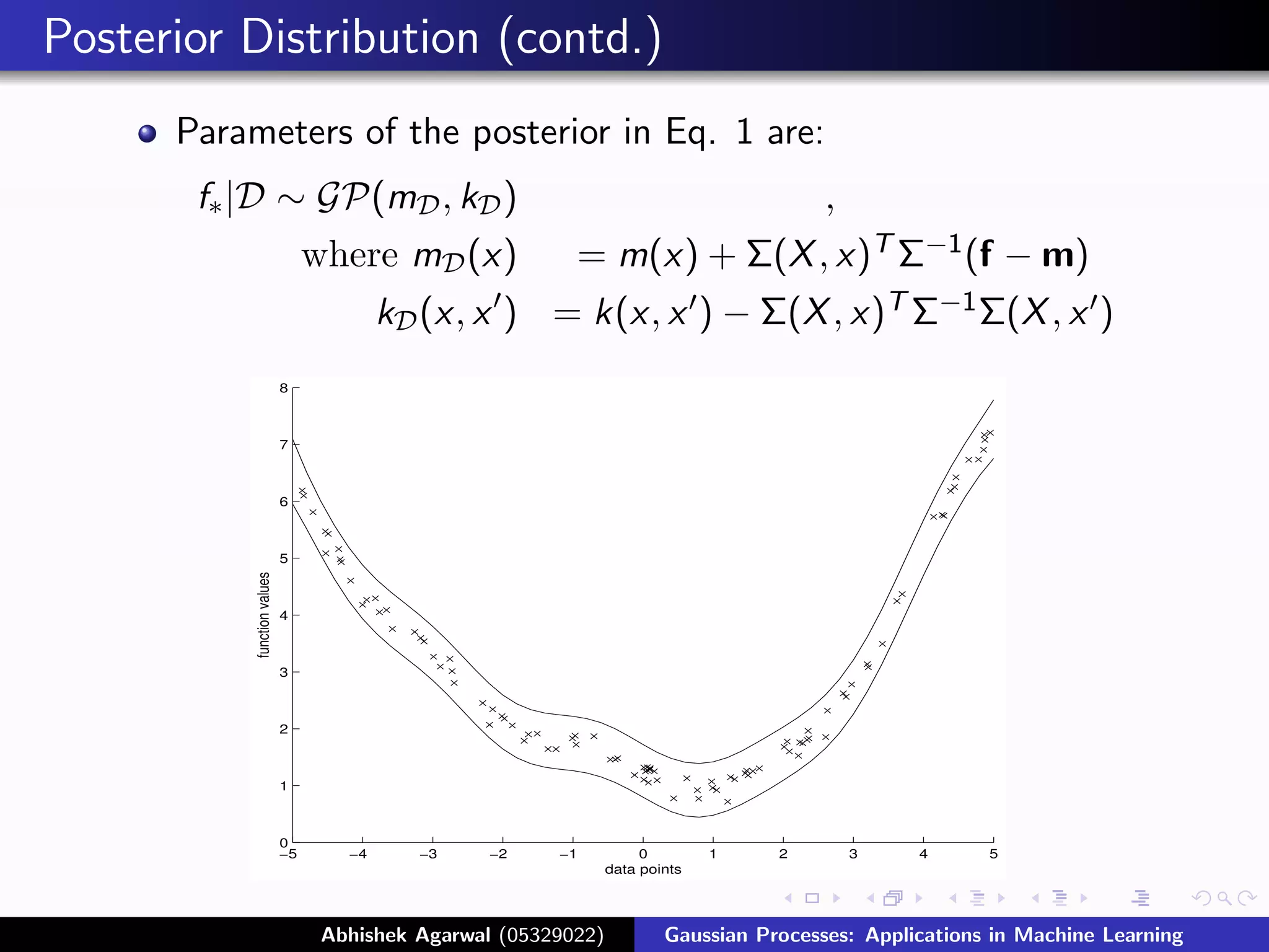
8. Posterior Distribution (contd.)
Parameters of the posterior in Eq. 1 are:
f∗ |D ∼ GP(mD , kD ) ,
where mD (x) = m(x) + Σ(X , x)T Σ−1 (f − m)
kD (x, x ) = k(x, x ) − Σ(X , x)T Σ−1 Σ(X , x )
8
7
6
5
function values
4
3
2
1
0
−5 −4 −3 −2 −1 0 1 2 3 4 5
data points
Figure: Prediction from GP Applications in Machine Learning
Abhishek Agarwal (05329022)
Gaussian Processes:

9. GP Models: Regression
GP can be directly applied to Bayesian Linear Regression
model like:
f (x) = φ(x)T w with prior w ∼ N (0, Σ)
Parameters for this distribution will be:
E[f (x)] = φ(x)T E[w ] = 0,
E[f (x)f (x )] = φ(x)T E[ww T ]φ(x ) = φ(x)T Σp φ(x )
So, f (x) and f (x ) are jointly Gaussian with zero mean and
covariance φ(x)T Σp φ(x ).
Abhishek Agarwal (05329022) Gaussian Processes: Applications in Machine Learning

10. GP Models: Regression (contd.)
In Regression, posterior distribution over the weights, is given
as (9):
likelhood ∗ prior
posterior =
marginal likelihood
Both prior p(f|X ) and likelihood p(y |f, X ) are Gaussian:
prior: f|X ∼ N (0, K ) (5)
likelihood: y|f ∼ N (f, σ n 2 I)
Marginal Likelihood p(y |X ) is defined as (6):
p(y |X ) = p(y |f, X )p(f|X )df (2)
Abhishek Agarwal (05329022) Gaussian Processes: Applications in Machine Learning

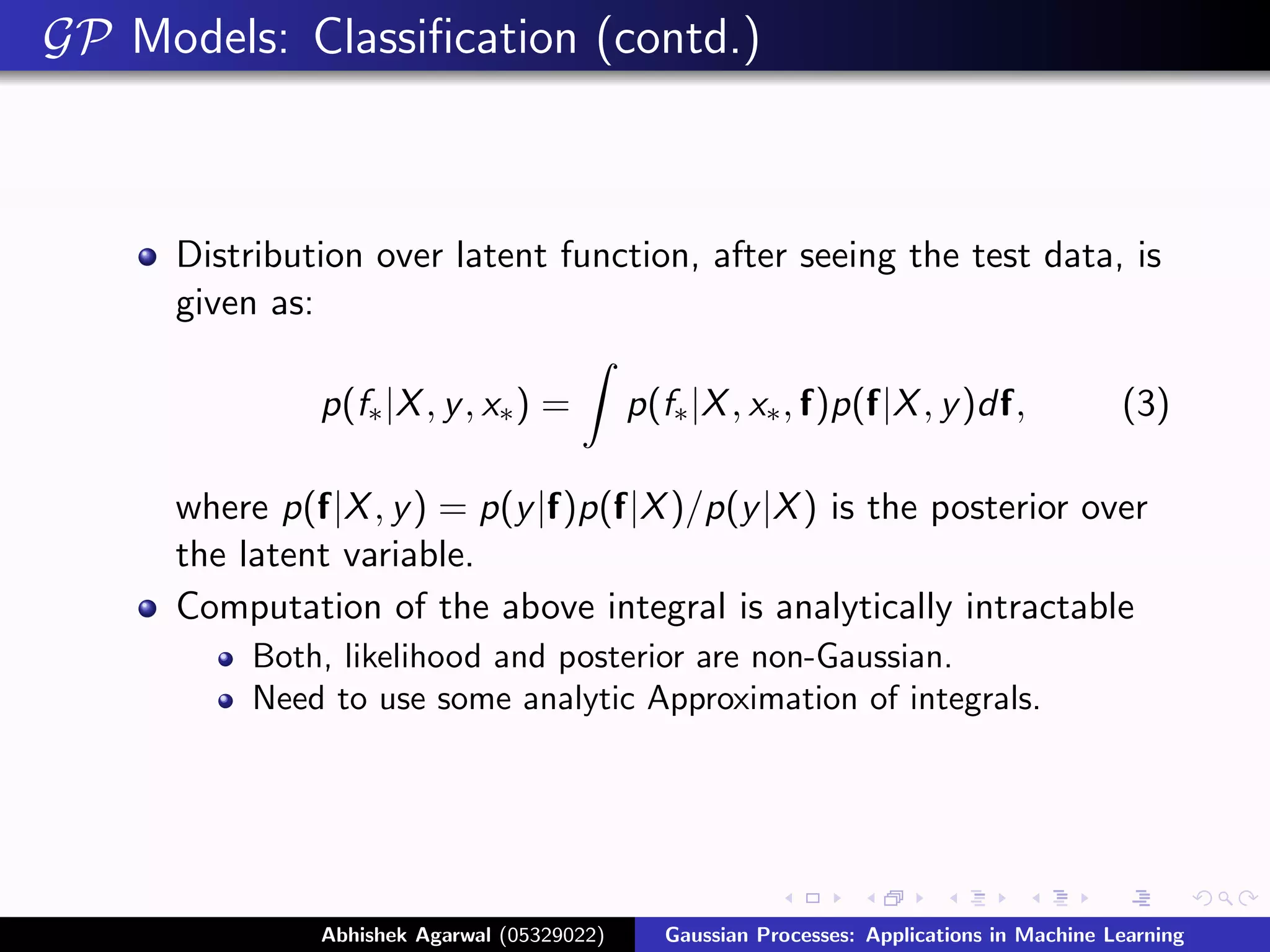
11. GP Models: Classification
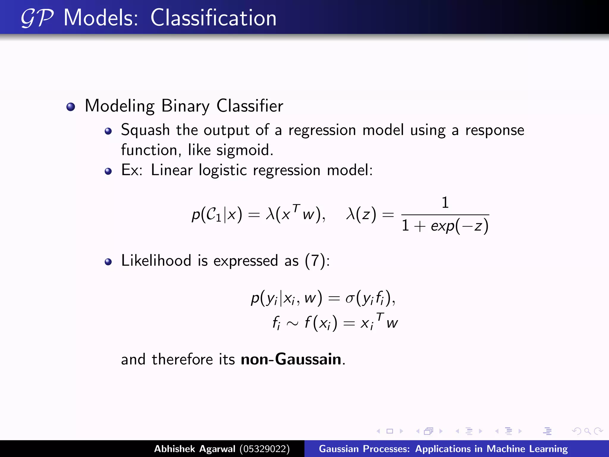
Modeling Binary Classifier
Squash the output of a regression model using a response
function, like sigmoid.
Ex: Linear logistic regression model:
1
p(C1 |x) = λ(x T w ), λ(z) =
1 + exp(−z)
Likelihood is expressed as (7):
p(yi |xi , w ) = σ(yi fi ),
fi ∼ f (xi ) = x i T w
and therefore its non-Gaussain.
Abhishek Agarwal (05329022) Gaussian Processes: Applications in Machine Learning

12. GP Models: Classification (contd.)
Distribution over latent function, after seeing the test data, is
given as:
p(f∗ |X , y , x∗ ) = p(f∗ |X , x∗ , f)p(f|X , y )df, (3)
where p(f|X , y ) = p(y |f)p(f|X )/p(y |X ) is the posterior over
the latent variable.
Computation of the above integral is analytically intractable
Both, likelihood and posterior are non-Gaussian.
Need to use some analytic Approximation of integrals.
Abhishek Agarwal (05329022) Gaussian Processes: Applications in Machine Learning

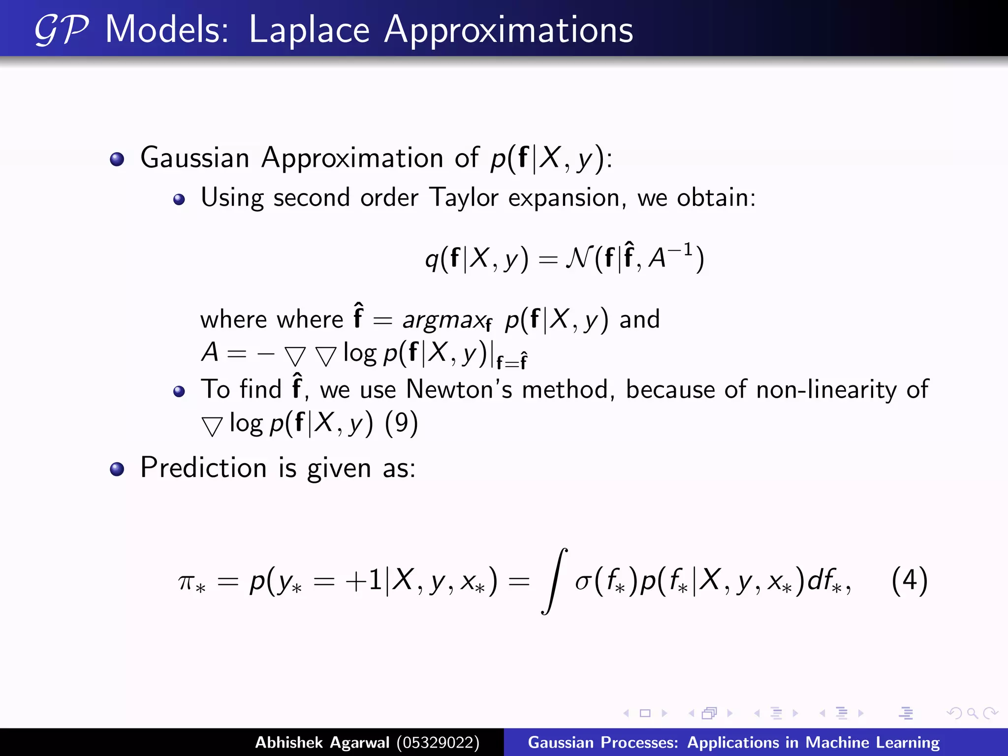
13. GP Models: Laplace Approximations
Gaussian Approximation of p(f|X , y ):
Using second order Taylor expansion, we obtain:
q(f|X , y ) = N (f|ˆ A−1 )
f,
where where ˆ = argmaxf p(f|X , y ) and
f
A=− log p(f|X , y )|f=ˆ
f
To find ˆ we use Newton’s method, because of non-linearity of
f,
log p(f|X , y ) (9)
Prediction is given as:
π∗ = p(y∗ = +1|X , y , x∗ ) = σ(f∗ )p(f∗ |X , y , x∗ )df∗ , (4)
Abhishek Agarwal (05329022) Gaussian Processes: Applications in Machine Learning

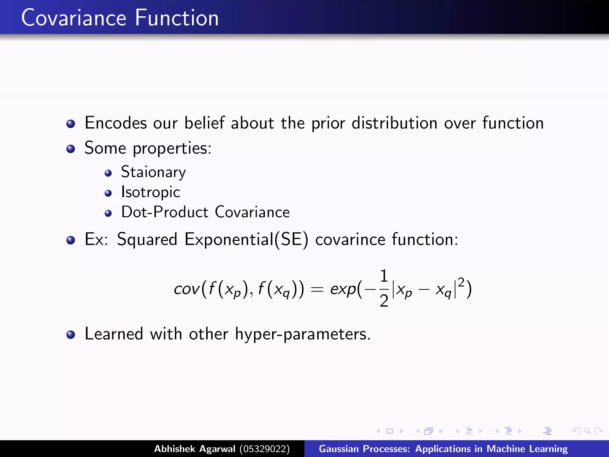
14. Covariance Function
Encodes our belief about the prior distribution over function
Some properties:
Staionary
Isotropic
Dot-Product Covariance
Ex: Squared Exponential(SE) covarince function:
1
cov (f (xp ), f (xq )) = exp(− |xp − xq |2 )
2
Learned with other hyper-parameters.
Abhishek Agarwal (05329022) Gaussian Processes: Applications in Machine Learning

15. Summary and Future Work
Current Research:
Fast sparse approximation algorithm for matrix inversion.
Approximation algorithm for non-Gaussian likelihoods.
GP approach has outperformed traditional methods in many
applications.
Gaussin Process based Positioning System (GPPS) [6]
Multi user Detection (MUD) in CDMA [7]
GP models are more powerful and flexible than simple
linear parametric models and less complex in comparison
to other models like multi-layer perceptrons. [1]
Abhishek Agarwal (05329022) Gaussian Processes: Applications in Machine Learning

16. Rasmussen and Williams. Gaussian Process for Machine
Learning, The MIT Press, 2006.
Matthias Seeger. Gaussian Process for Machine Learning,
2004. International Journal of Neural Systems, 14(2):69-106,
2004.
Christopher Williams, Bayesian Classification with Gaussian
Processes, In IEEE Trans. Pattern analysis and Machine
Intelligence, 1998
Rasmussen and Williams, Gaussian Process for Regression. In
Proceedings of NIPS’ 1996.
Rasmussen, Evaluation of Gaussian Processes and Other
Methods for Non-linear Regression. PhD thesis, Dept. of
Computer Science, University of Toronto, 1996. Available from
http://www.cs.utoronto.ca/ carl/
Abhishek Agarwal (05329022) Gaussian Processes: Applications in Machine Learning

17. Anton Schwaighofer, et. al. GPPS: A Gaussian Process
Positioning System for Cellular Networks, In proceedings of
NIPS’ 2003.
Murillo-Fuentes, et. al. Gaussian Processes for Multiuser
Detection in CDMA receivers, Advances in Neural Information
Processing System’ 2005
David Mackay, Introduction to Gaussian Processes
C. Williams. Gaussian processes. In M. A. Arbib, editor,
Handbook of Brain Theory and Neural Networks, pages
466-470. The MIT Press, second edition, 2002.
Abhishek Agarwal (05329022) Gaussian Processes: Applications in Machine Learning

18. Thank You !!
Questions ??
Abhishek Agarwal (05329022) Gaussian Processes: Applications in Machine Learning

19. Extra
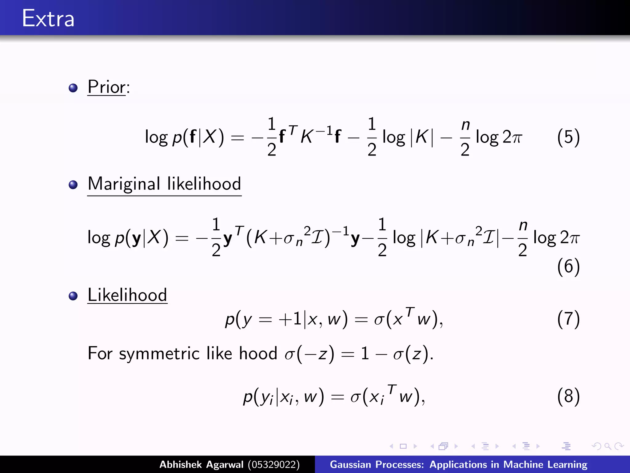
Prior:
1 1 n
log p(f|X ) = − f T K −1 f − log |K | − log 2π (5)
2 2 2
Mariginal likelihood
1 1 n
log p(y|X ) = − yT (K +σ n 2 I)−1 y− log |K +σ n 2 I|− log 2π
2 2 2
(6)
Likelihood
p(y = +1|x, w ) = σ(x T w ), (7)
For symmetric like hood σ(−z) = 1 − σ(z).
p(yi |xi , w ) = σ(x i T w ), (8)
Abhishek Agarwal (05329022) Gaussian Processes: Applications in Machine Learning

20. Extra (contd.)
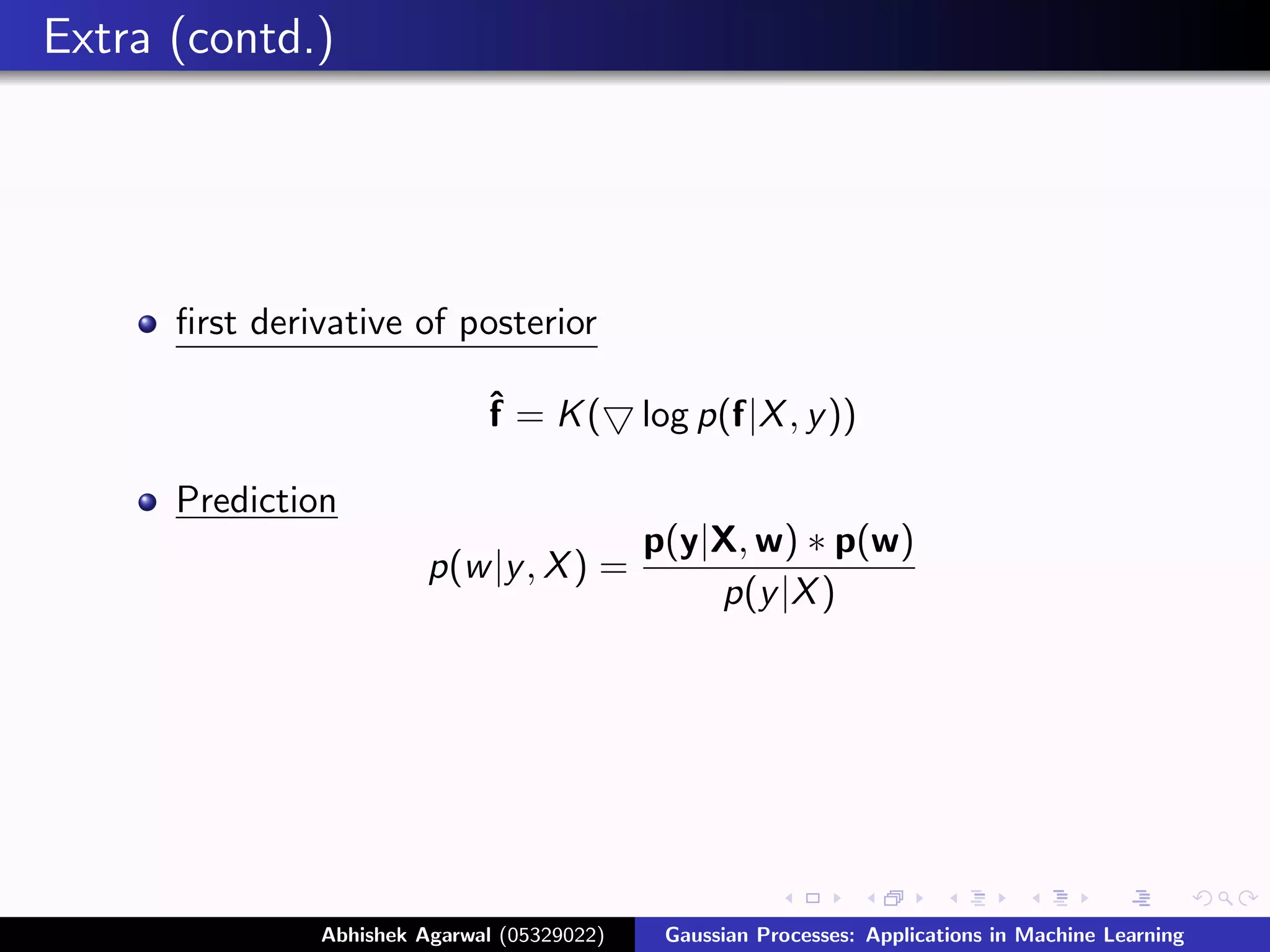
first derivative of posterior
ˆ = K(
f log p(f|X , y ))
Prediction
p(y|X, w) ∗ p(w)
p(w |y , X ) =
p(y |X )
Abhishek Agarwal (05329022) Gaussian Processes: Applications in Machine Learning