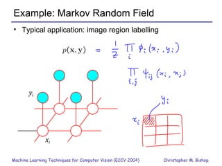
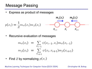
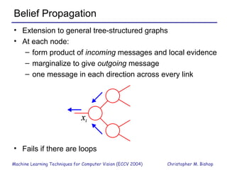
Part 1 of the document provides an overview of graphical models and machine learning techniques for computer vision. It discusses directed and undirected graphs, inference using message passing algorithms like belief propagation, and learning techniques like maximum likelihood and Bayesian learning. Graphical models allow modeling complex distributions and exploiting conditional independencies between variables. Inference on graphs is generally intractable for large cliques, but approximations like loopy belief propagation are commonly used.

1. Part 1: Graphical Models Machine Learning Techniques for Computer Vision Microsoft Research Cambridge ECCV 2004, Prague Christopher M. Bishop

2. About this Tutorial Learning is the new frontier in computer vision Focus on concepts not lists of algorithms not technical details Graduate level Please ask questions!

3. Overview Part 1: Graphical models directed and undirected graphs inference and learning Part 2: Unsupervised learning mixture models, EM variational inference, model complexity continuous latent variables Part 3: Supervised learning decision theory linear models, neural networks, boosting, sparse kernel machines

4. Probability Theory Sum rule Product rule From these we have Bayes’ theorem with normalization

5. Role of the Graphs New insights into existing models Motivation for new models Graph based algorithms for calculation and computation c.f. Feynman diagrams in physics

6. Decomposition Consider an arbitrary joint distribution By successive application of the product rule

7. Directed Acyclic Graphs Joint distribution where denotes the parents of i No directed cycles

8. Undirected Graphs Provided then joint distribution is product of non-negative functions over the cliques of the graph where are the clique potentials, and Z is a normalization constant

9. Conditioning on Evidence Variables may be hidden (latent) or visible (observed) Latent variables may have a specific interpretation, or may be introduced to permit a richer class of distribution

10. Conditional Independences x independent of y given z if, for all values of z , For undirected graphs this is given by graph separation!

11. “Explaining Away” C.I. for directed graphs similar, but with one subtlety Illustration: pixel colour in an image image colour surface colour lighting colour

12. Directed versus Undirected

13. Example: State Space Models Hidden Markov model Kalman filter

14. Example: Bayesian SSM

15. Example: Factorial SSM Multiple hidden sequences Avoid exponentially large hidden space

16. Example: Markov Random Field Typical application: image region labelling

17. Example: Conditional Random Field

18. Inference Simple example: Bayes’ theorem

19. Message Passing Example Find marginal for a particular node for M -state nodes, cost is exponential in length of chain but, we can exploit the graphical structure (conditional independences)

20. Message Passing Joint distribution Exchange sums and products

21. Message Passing Express as product of messages Recursive evaluation of messages Find Z by normalizing

22. Belief Propagation Extension to general tree-structured graphs At each node: form product of incoming messages and local evidence marginalize to give outgoing message one message in each direction across every link Fails if there are loops

23. Junction Tree Algorithm An efficient exact algorithm for a general graph applies to both directed and undirected graphs compile original graph into a tree of cliques then perform message passing on this tree Problem: cost is exponential in size of largest clique many vision models have intractably large cliques

24. Loopy Belief Propagation Apply belief propagation directly to general graph need to keep iterating might not converge State-of-the-art performance in error-correcting codes

25. Max-product Algorithm Goal: find define then Message passing algorithm with “sum” replaced by “max” Example: Viterbi algorithm for HMMs

26. Inference and Learning Data set Likelihood function (independent observations) Maximize (log) likelihood Predictive distribution

27. Regularized Maximum Likelihood Prior , posterior MAP (maximum posterior) Predictive distribution Not really Bayesian

28. Bayesian Learning Key idea is to marginalize over unknown parameters, rather than make point estimates avoids severe over-fitting of ML and MAP allows direct model comparison Parameters are now latent variables Bayesian learning is an inference problem!

29. Bayesian Learning

30. Bayesian Learning

31. And Finally … the Exponential Family Many distributions can be written in the form Includes: Gaussian Dirichlet Gamma Multi-nomial Wishart Bernoulli … Building blocks in graphs to give rich probabilistic models

32. Illustration: the Gaussian Use precision (inverse variance) In standard form

33. Maximum Likelihood Likelihood function (independent observations) Depends on data via sufficient statistics of fixed dimension

34. Conjugate Priors Prior has same functional form as likelihood Hence posterior is of the form Can interpret prior as effective observations of value Examples: Gaussian for the mean of a Gaussian Gaussian-Wishart for mean and precision of Gaussian Dirichlet for the parameters of a discrete distribution

35. Summary of Part 1 Directed graphs Undirected graphs Inference by message passing: belief propagation