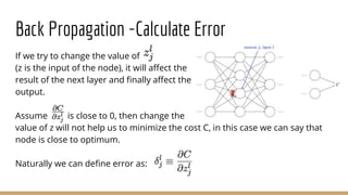
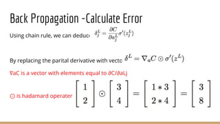
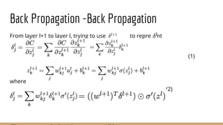
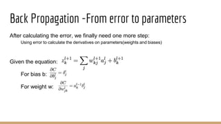
Downloaded 26 times
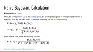
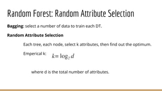
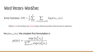
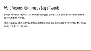
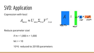
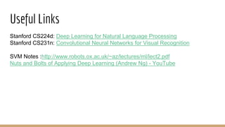
![Recurrent Neural Network-Loss Function
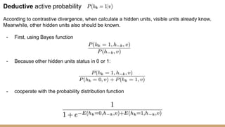
The cross-entropy in one single time step:
Overall cross-entrophy cost:
Where V is the vocabulary and T means the text.
Exp:
yt = [0.3,0.6,0.1] the, a, movie
y1 = [0.001,0.009,0.9]
y2 = [0.001,0.299,0.7]
y3 = [0.001,0.9,0.009]
J1= yt*logJ1
J2= yt*logJ2
J3 = yt*logJ3
J3>J2>J1 because y3 is more close to
yt than others.](https://image.slidesharecdn.com/mlpart2draft-170327101428/85/Machine-Learning-Algorithms-Review-Part-2-72-320.jpg)
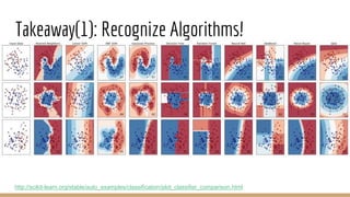
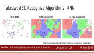

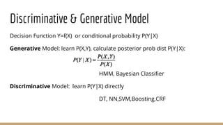
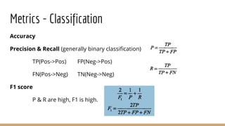
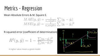
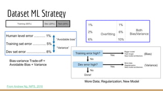
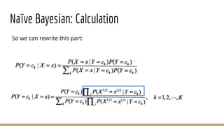
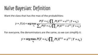
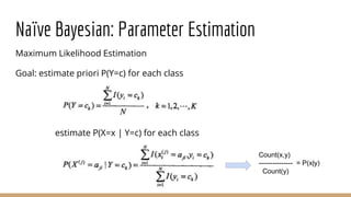
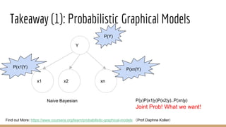
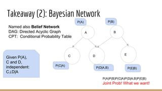
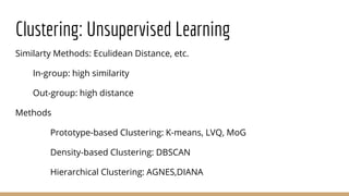
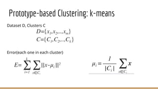
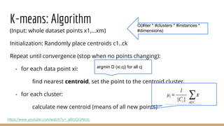
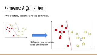
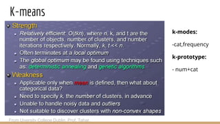
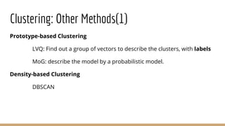
This document provides an overview of machine learning algorithms and techniques. It discusses classification and regression metrics, naive Bayesian classifiers, clustering methods like k-means, ensemble learning techniques like bagging and boosting, the expectation maximization algorithm, restricted Boltzmann machines, neural networks including convolutional and recurrent neural networks, and word embedding techniques like Word2Vec, GloVe, and matrix factorization. Key algorithms and their applications are summarized at a high level.