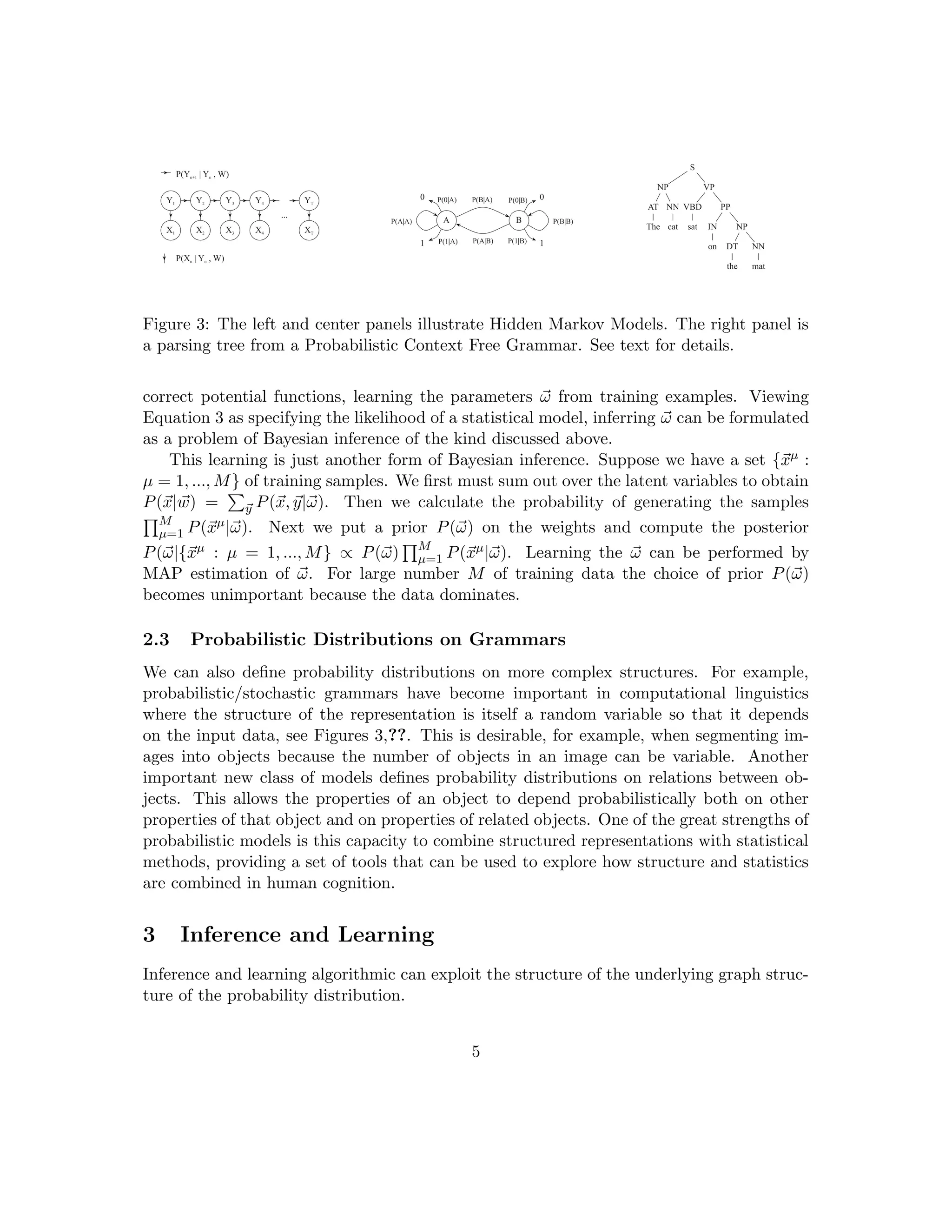
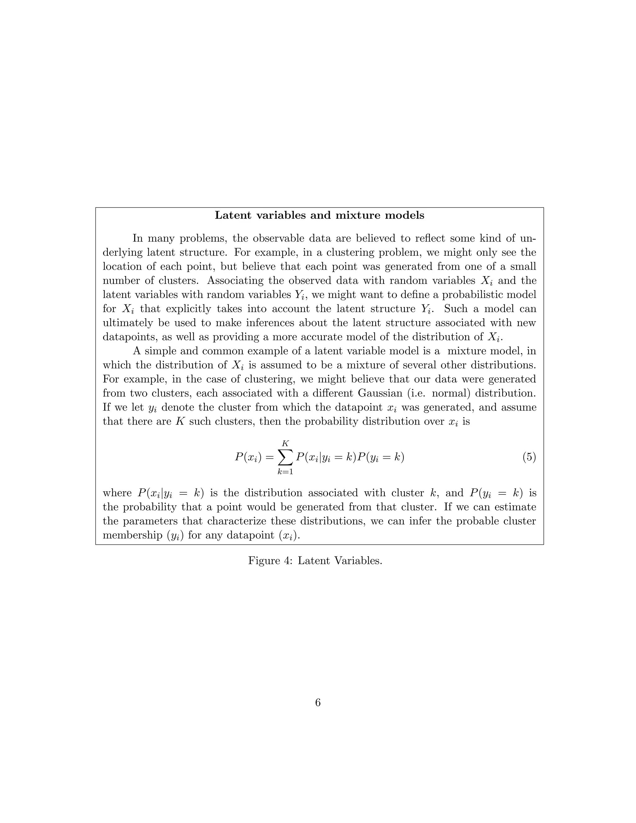
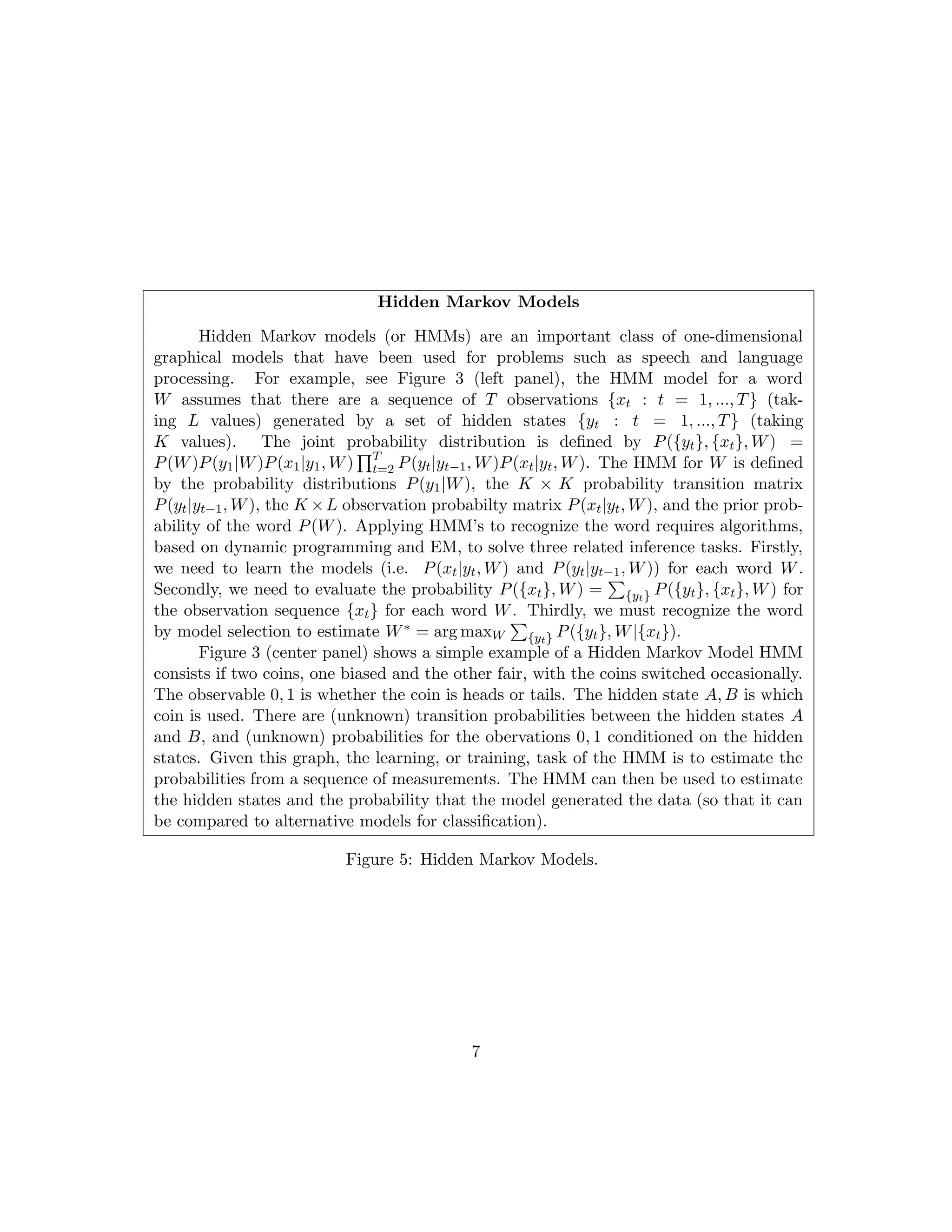
The document discusses probabilistic models and graphical models for understanding dependencies among variables. It covers directed graphical models (Bayesian networks) and undirected graphical models (Markov Random Fields), detailing their structures, relationships, and implications for probabilistic inference and learning. Examples include applications in vision, hidden Markov models, mixture models, and probabilistic context-free grammars.

1. Lecture 15. Probabilistic Models on Graph
Prof. Alan Yuille
Spring 2014
1 Introduction
We discuss how to define probabilistic models that use richly structured probability dis-
tributions and describe how graphical models can be used to represent the dependencies
among a set of variables. Then we describe dynamic programming and EM for learning.
2 Representing structured probability distributions
A probabilistic model defines the joint distribution for a set of random variables. For
example, imagine that a friend of yours claims to possess psychic powers – in particular,
the power of psychokinesis. He proposes to demonstrate these powers by flipping a coin,
and influencing the outcome to produce heads. You suggest that a better test might be to
see if he can levitate a pencil, since the coin producing heads could also be explained by
some kind of sleight of hand, such as substituting a two-headed coin. We can express all
possible outcomes of the proposed tests, as well as their causes, using the binary random
variables X1, X2, X3, and X4 to represent (respectively) the truth of the coin being flipped
and producing heads, the pencil levitating, your friend having psychic powers, and the
use of a two-headed coin. Any set of beliefs about these outcomes can be encoded in a
joint probability distribution, P(x1, x2, x3, x4). For example, the probability that the coin
comes up heads (x1 = 1) should be higher if your friend actually does have psychic powers
(x3 = 1).
Once we have defined a joint distribution on X1, X2, X3, and X4, we can reason
about the implications of events involving these variables. For example, if flipping the coin
produces heads (x1 = 1), then the probability distribution over the remaining variables is
P(x2, x3, x4|x1 = 1) =
P(x1 = 1, x2, x3, x4)
P(x1 = 1)
. (1)
This equation can be interpreted as an application of Bayes’ rule, with X1 being the data,
and X2, X3, X4 being the hypotheses. However, in this setting, as with most probabilistic
models, any variable can act as data or hypothesis. In the general case, we use probabilistic
1

2. inference to compute the probability distribution over a set of unobserved variables (here,
X2, X3, X4) conditioned on a set of observed variables (here, X1).
4
coin produces heads
two−headed coin
pencil levitates
friend has psychic powers
X
X1
X3
X2
Figure 1: Directed graphical model (Bayes net) showing the dependencies among variables
in the “psychic friend” example discussed in the text.
Another common pattern of influence is explaining away. Imagine that your friend
flipped the coin, and it came up heads (x1 = 1). The propositions that he has psychic
powers (x3 = 1) and that it is a two-headed coin (x4 = 1) might both become more
likely. However, while these two variables were independent before seeing the outcome of
the coinflip, they are now dependent: if you were to go on to discover that the coin has
two heads, the hypothesis of psychic powers would return to its baseline probability – the
evidence for psychic powers was “explained away” by the presence of the two-headed coin.
2.1 Directed graphical models
Directed graphical models, also known as Bayesian networks or Bayes nets, consist of a
set of nodes, representing random variables, together with a set of directed edges from one
node to another, which can be used to identify statistical dependencies between variables.
Typically, nodes are drawn as circles, and the existence of a directed edge from one node to
another is indicated with an arrow between the corresponding nodes. If an edge exists from
node A to node B, then A is referred to as the “parent” of B, and B is the “child” of A.
This genealogical relation is often extended to identify the “ancestors” and “descendants”
of a node.
The directed graph used in a Bayes net has one node for each random variable in
the associated probability distribution. The edges express the statistical dependencies
between the variables in a fashion consistent with the Markov condition: conditioned
on its parents, each variable is independent of all other variables except its descendants.
This has an important implication: a Bayes net specifies a canonical factorization of a
probability distribution into the product of the conditional distribution for each variable
conditioned on its parents. Thus, for a set of variables X1, X2, . . . , XM , we can write
P(x1, x2, . . . , xM ) =
Q
i P(xi|Pa(Xi)) where Pa(Xi) is the set of parents of Xi.
2

3. Figure 1 shows a Bayes net for the example of the friend who claims to have psychic pow-
ers. This Bayes net identifies a number of assumptions about the relationship between the
variables involved in this situation. For example, X1 and X2 are assumed to be independent
given X3, indicating that once it was known whether or not your friend was psychic, the
outcomes of the coin flip and the levitation experiments would be completely unrelated. By
the Markov condition, we can write P(x1, x2, x3, x4) = P(x1|x3, x4)P(x2|x3)P(x3)P(x4).
This factorization allows us to use fewer numbers in specifying the distribution over these
four variables: we only need one number for each variable, conditioned on each set of values
taken on by its parents. In this case, this adds up to 8 numbers rather than 15.
2.2 Undirected graphical models
Undirected graphical models, also known as Markov Random Fields (MRFs), consist of
a set of nodes, representing random variables, and a set of undirected edges, defining
neighbourhood structure on the graph which indicates the probabilistic dependencies of the
variables at the nodes. Each set of fully-connected neighbors as associated with a potential
function, which varies as the associated random variables take on different values. When
multiplied together, these potential functions give the probability distribution over all the
variables. Unlike directed graphical models, there need be no simple relationship between
these potentials and the local conditional probability distributions. Moreover, undirected
graphical models usually have closed loops (if they do not, then they can be reformulated
as directed graphical models).
In this section we will use Xi to refer to variables whose values can be directed ob-
served and Yi to refer to latent, or hidden, variables whose values can only be inferred, see
figure (4). We will use the vector notation ~
x and ~
y to represent the values taken by these
random variables, being x1, x2, . . . and y1, y2, . . . respectively.
A standard model used in vision is of form: P(~
x|~
y) = (
Q
i P(xi|yi)) P(~
y) where the
prior distribution on the latent variables is an MRF,
P(~
y) =
1
Z
Y
i,j∈Λ
ψij(yi, yj)
Y
i
ψi(yi) (2)
where Z is a normalizing constant ensuring that the resulting distribution sums to 1. Here,
ψij(·, ·) and ψi(·) are the potential functions, and the underlying graph is a lattice, with Λ
being the set of connected pairs of nodes (see Figure 2). This model has many applications.
For example, ~
x can be taken to be the observed intensity values of a corrupted image and
~
y the true image intensity, with P(xi|yi) modeling the corruption of these intensity values.
The prior P(~
y) is used to put prior probabilities on the true intensity, for example that
neighbouring intensity values are similar (e.g. that the intensity is spatially smooth). A
similar model can be used for binocular stereopsis, where the ~
x correspond to the image
intensities in the left and right eyes and ~
y denotes the depth of the surface in space that
3

4. Figure 2: The left panel illustrates an MRF model where Λ = {(1, 2), (2, 3), (3, 4), (4, 1)},
see text for more details. The right panel is a Boltzmann Machine, see text for details.
generates the two images. The prior on ~
y can assume that the depth is a spatially smoothly
varying function.
The neighbourhood structure, given by Λ above, will typically correspond to a graph
structure with closed loops, see figure. A graph with no closed loops is called a tree. It
can easily be shown that an undirected graphical model on a tree can be reformulated as a
directed graphical model on the same tree. This will make it significantly easier to perform
inference, see next section. Tree models occur naturally for problems whose structure is
one-dimensional such as speech recognition. See Hidden Markov Models in figure (5). For
vision problems, however, undirected graphical models will be defined on graphs with closed
loops. In this case inference becomes more difficult and requires more complex algorithms
that we describe in the next section.
Another example of an MRF is the Boltzmann Machine, which has been very influential
in the neural network community. In this model the components xi and yi of the observed
and latent variables ~
x and ~
y all take on values 0 or 1. The standard model is
P(~
y, ~
x|~
ω) =
1
Z
exp{−E(~
y, ~
x, ~
ω)/T} (3)
where T is a parameter reflecting the “temperature” of the system, and E depends on
unknown parameters ~
ω which are weighted connections ωh
ij between hidden variables yi, yj
and ωo
ij between observed and hidden variables xi, yj,
E(~
y, ~
x, ~
ω) =
X
ij
ωo
ijxiyj +
X
ij
ωh
ijyiyj. (4)
In this model, the potential functions are of the form exp{−ωo
ijxiyj} and exp{−ωh
ijyiyj},
and the underlying graph connects pairs of observed and hidden variables and pairs of
hidden variables (see Figure 2). Training the Boltzmann Machine involves identifying the
4

5. Figure 3: The left and center panels illustrate Hidden Markov Models. The right panel is
a parsing tree from a Probabilistic Context Free Grammar. See text for details.
correct potential functions, learning the parameters ~
ω from training examples. Viewing
Equation 3 as specifying the likelihood of a statistical model, inferring ~
ω can be formulated
as a problem of Bayesian inference of the kind discussed above.
This learning is just another form of Bayesian inference. Suppose we have a set {~
xµ :
µ = 1, ..., M} of training samples. We first must sum out over the latent variables to obtain
P(~
x|~
w) =
P
~
y P(~
x, ~
y|~
ω). Then we calculate the probability of generating the samples
QM
µ=1 P(~
xµ|~
ω). Next we put a prior P(~
ω) on the weights and compute the posterior
P(~
ω|{~
xµ : µ = 1, ..., M} ∝ P(~
ω)
QM
µ=1 P(~
xµ|~
ω). Learning the ~
ω can be performed by
MAP estimation of ~
ω. For large number M of training data the choice of prior P(~
ω)
becomes unimportant because the data dominates.
2.3 Probabilistic Distributions on Grammars
We can also define probability distributions on more complex structures. For example,
probabilistic/stochastic grammars have become important in computational linguistics
where the structure of the representation is itself a random variable so that it depends
on the input data, see Figures 3,??. This is desirable, for example, when segmenting im-
ages into objects because the number of objects in an image can be variable. Another
important new class of models defines probability distributions on relations between ob-
jects. This allows the properties of an object to depend probabilistically both on other
properties of that object and on properties of related objects. One of the great strengths of
probabilistic models is this capacity to combine structured representations with statistical
methods, providing a set of tools that can be used to explore how structure and statistics
are combined in human cognition.
3 Inference and Learning
Inference and learning algorithmic can exploit the structure of the underlying graph struc-
ture of the probability distribution.
5

6. Latent variables and mixture models
In many problems, the observable data are believed to reflect some kind of un-
derlying latent structure. For example, in a clustering problem, we might only see the
location of each point, but believe that each point was generated from one of a small
number of clusters. Associating the observed data with random variables Xi and the
latent variables with random variables Yi, we might want to define a probabilistic model
for Xi that explicitly takes into account the latent structure Yi. Such a model can
ultimately be used to make inferences about the latent structure associated with new
datapoints, as well as providing a more accurate model of the distribution of Xi.
A simple and common example of a latent variable model is a mixture model, in
which the distribution of Xi is assumed to be a mixture of several other distributions.
For example, in the case of clustering, we might believe that our data were generated
from two clusters, each associated with a different Gaussian (i.e. normal) distribution.
If we let yi denote the cluster from which the datapoint xi was generated, and assume
that there are K such clusters, then the probability distribution over xi is
P(xi) =
K
X
k=1
P(xi|yi = k)P(yi = k) (5)
where P(xi|yi = k) is the distribution associated with cluster k, and P(yi = k) is
the probability that a point would be generated from that cluster. If we can estimate
the parameters that characterize these distributions, we can infer the probable cluster
membership (yi) for any datapoint (xi).
Figure 4: Latent Variables.
6

7. Hidden Markov Models
Hidden Markov models (or HMMs) are an important class of one-dimensional
graphical models that have been used for problems such as speech and language
processing. For example, see Figure 3 (left panel), the HMM model for a word
W assumes that there are a sequence of T observations {xt : t = 1, ..., T} (tak-
ing L values) generated by a set of hidden states {yt : t = 1, ..., T} (taking
K values). The joint probability distribution is defined by P({yt}, {xt}, W) =
P(W)P(y1|W)P(x1|y1, W)
QT
t=2 P(yt|yt−1, W)P(xt|yt, W). The HMM for W is defined
by the probability distributions P(y1|W), the K × K probability transition matrix
P(yt|yt−1, W), the K ×L observation probabilty matrix P(xt|yt, W), and the prior prob-
ability of the word P(W). Applying HMM’s to recognize the word requires algorithms,
based on dynamic programming and EM, to solve three related inference tasks. Firstly,
we need to learn the models (i.e. P(xt|yt, W) and P(yt|yt−1, W)) for each word W.
Secondly, we need to evaluate the probability P({xt}, W) =
P
{yt} P({yt}, {xt}, W) for
the observation sequence {xt} for each word W. Thirdly, we must recognize the word
by model selection to estimate W∗ = arg maxW
P
{yt} P({yt}, W|{xt}).
Figure 3 (center panel) shows a simple example of a Hidden Markov Model HMM
consists if two coins, one biased and the other fair, with the coins switched occasionally.
The observable 0, 1 is whether the coin is heads or tails. The hidden state A, B is which
coin is used. There are (unknown) transition probabilities between the hidden states A
and B, and (unknown) probabilities for the obervations 0, 1 conditioned on the hidden
states. Given this graph, the learning, or training, task of the HMM is to estimate the
probabilities from a sequence of measurements. The HMM can then be used to estimate
the hidden states and the probability that the model generated the data (so that it can
be compared to alternative models for classification).
Figure 5: Hidden Markov Models.
7

8. Box 5: Probabilistic Context Free Grammars
A probabilistic context free grammar (or PCFG) is a context free grammar that
associates a probability with each of its production rules. A PCFG can be used to
generate sentences and to parse them. The probability of a sentence, or a parse, is
defined to be the product of the probabilities of the production rules used to generate
the sentence.
For example, we define a PCFG to generate a parse tree as
follows, see Figure 3 (right panel). We define non-terminal nodes
S, NP, V P, AT, NNS, V BD, PP, IN, DT, NN where S is a sentence, V P is a verb
phrase, V BD is a verb,NP is a noun phrase, NN is a noun, and so on. The terminal
nodes are words from a dictionary (e.g. “the”, “cat”, “sat”, “on”, “mat”.) We define
production rules which are applied to non-terminal nodes to generate child nodes (e.g.
S 7→ NP, V P or NN 7→ “cat”). We specify probabilities for the production rules.
These production rules enable us to generate a sentence starting from the root
node S. We sample to select a production rule and apply it to generate child nodes. We
repeat this process on the child nodes and stop when all the nodes are terminal (i.e. all
are words). To parse an input sentence, we use dynamic programming to compute the
most probable way the sentence could have been generated by the production rules.
We can learn the production rules, and their probabilities, from training data of
sentences. This can be done in a supervised way, where the correct parsing the sentences
is known. Or in an unsupervised way, as described by Klein and Manning.
Probabilistic context free grammars have several important features. Firstly, the
number of nodes in these graphs are variable (unlike other models where the number of
nodes is fixed). Moreover, they have independence properties so that different parts of
the tree are independent. This is, at best, an approximation for natural language and
more complex models are needed.
Figure 6: Probabilistic Context Free Grammars.
8

9. Figure 7: Examples of Dynamic Programming.
3.1 Dynamic Programming for Inference
In particular, if the underlying graph is a tree (i.e. it has no closed loops), dynamic
programming (DP) algorithms can be used to exploit this structure, see figure 7. The
intuition behind DP can be illustrated by planning the shortest route for a trip from Los
Angeles to Boston. To determine the cost of going via Chicago, you only need to calculate
the shortest route from LA to Chicago and then, independently, from Chicago to Boston.
Decomposing the route in this way, and taking into account the linear nature of the trip,
gives an efficient algorithm with convergence rates which are polynomial in the number of
nodes and hence are often feasible for computation. Equation (7) is one illustration for
how the dynamic programming can exploit the structure of the problem to simplify the
computation. These methods are put to particularly good use in hidden Markov models,
see figure 5.
Dynamic Programming can be used when we can express the graph as a tree structure
and hence order the nodes.
P(~
y) =
1
Z
N−1
Y
i=1
ψi(yi, yi+1)
N−1
Y
i=1
ψi(yi) (6)
We maximize equation (6) with respect to y by using the max rule version of dynamic
programming. This can be done recursively by defining a function hi(yi) by a phforward
pass:
hi(yi) = max
yi−1
hi−1(yi−1)ψi(yi−1, yi)ψi(yi), (7)
9

10. where h1(y1) = 1.
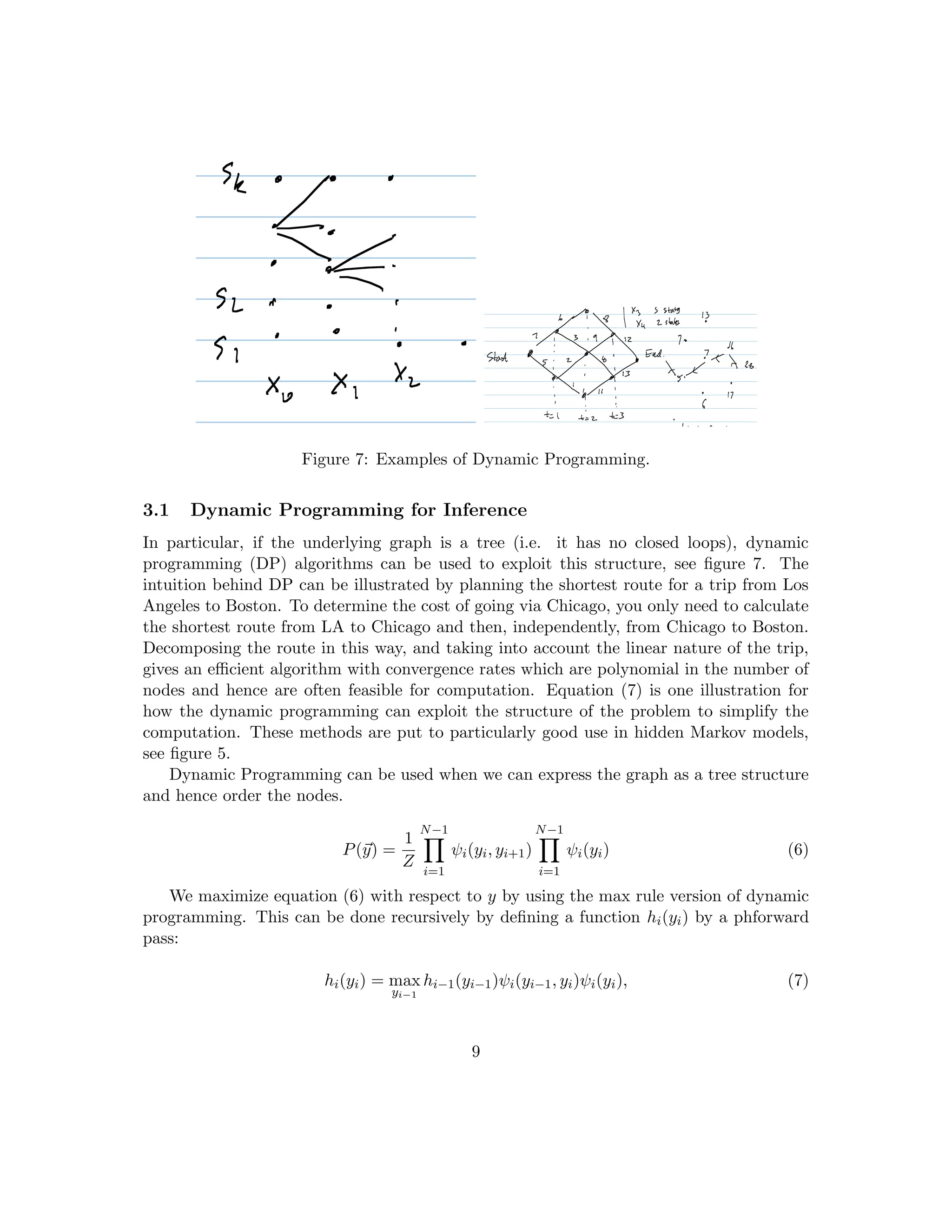
The forward pass computes the maximum value of P(~
y). The backward pass of dynamic
programming compute the most probable value ~
y∗.
The computational complexity of the dynamic programming algorithm is O(MNK)
where M is the number of cliques in the aspect model for the object, K = 2 is the size of
the maximum clique.
NOTE: WE CAN ALSO USE DYNAMIC PROGRAMMING TO COMPUTE THINGS
LIKE THE MARGINALS Pi(yi) and the PARTITION FUNCTION Z.
These are done by the sum-rule of dynamic programming – which replaces equation (7)
by
hi(yi) =
X
yi−1
hi−1(yi−1)ψi(yi−1, yi)ψi(yi). (8)
Dynamic programming can also be used for inference of probabilistic context free gram-
mars (PCFG).This is because the key idea of dynamic programming is independence – and
PCFGs produce trees where the different branches are independent of each other. Dynamic
Programming can only be applied directly to problems which are defined on tree structures
(because this allows us to order the nodes – the ordering does not have to be unique).
What if you do not have a tree structure (i.e., you have closed loops)? There is an
approach called junction trees which shows that you can transform any probability distri-
bution on a graph into a probability distribution on a tree by enhancing the variables. The
basic idea is triangulation (Lauritzen and Spiegelhalter). But this, while useful, is limited
because the resulting trees can be enormous.
3.2 EM and Dynamic Programming for Learning
Dynamic programming can also be used as a component of learning for models with latent
variables. Suppose we have a parameterized distribution P(~
x,~
h|λ) where ~
x is observed, ~
h
are the hidden states, and λ are the model parameters (to be learnt). The distribution
P(~
h) is an MRF. Given training data {~
xµ, µ = 1, ..., N} we should estimate λ by maximum
likelihood (ML) by computing:
λ∗
= arg max
λ
Y
µ
P(~
xµ|λ). (9)
P(~
xµ,~
hµ|λ) =
1
Z[λ]
exp(λ · φ(~
xµ,~
hµ))
For example, if the MRF of P(~
h) is a chain structure, we have
λ · φ(~
xµ,~
hµ) =
M
X
i=1
λu
i φ(x(i)
µ , h(i)
µ ) +
M−1
X
j=1
λp
j φ(h(j)
µ , h(j+1)
µ )
10

11. Note that both ~
xµ and ~
hµ are M-dimensional vector (the MRF has M nodes). λp
denotes parameters for pairwise terms and λu denotes parameters for unary terms.
If we can observe ~
hµ, then the MLE gives the optimal condition for λ
X
~
x,~
h
p(~
x,~
h|λ)φ(~
x,~
h) =
1
N
N
X
µ=1
φ(~
xµ,~
hµ).
In practice, we use steepest descent to compute the optimal λ iteratively.
Z[λ] =
X
~
x,~
h
exp(λ · φ(~
x,~
h))
F[λ] = log(Z[λ]) − λ ·
1
N
N
X
µ=1
φ(~
xµ,~
hµ)
λt+1
= λt
− γt ∂F[λ]
∂λ
λt+1
= λt
− γt
(
X
~
x,~
h
p(~
x,~
h|λ)φ(~
x,~
h) −
1
N
N
X
µ=1
φ(~
xµ,~
hµ)).
The summation over ~
h is done by dynamic programming.
However, ~
h is latent. So we have to use EM algorithm for learning. This requires
eliminating the hidden variables which is usually intractable analytically. Instead we can
apply the EM algorithm to minimize (local minima) a free energy:
F({qµ}, λ) =
X
µ
X
~
hµ
qµ(~
hµ) log qµ(~
hµ) −
X
µ
X
~
hµ
qµ(~
hµ) log P(~
xµ,~
hµ|λ). (10)
NOTE that we have distributions qµ(.) for the states ~
hµ of all training examples. But
the parameters λ are common for all examples.
The EM algorithm for equation (10) has the following E-step and M-step:
E − Step qt+1
µ (~
hµ) = P(~
hµ|~
xµ, λt
),
M − step λt+1
= arg min
X
µ
X
~
hµ
qt+1
µ (~
hµ) log P(~
xµ,~
hµ)|λ). (11)
There are two stages where dynamic programming helps makes the steps practical.
Firstly, computing P(~
hµ|~
xµ, λt) from P(~
h, ~
x|λ) (E-step) is practical because we can set
P(~
hµ|~
xµ, λt) ∝ P(~
h, ~
x|λ) and then use DP (sum-rule) to compute the normalization con-
stant. Secondly, the summation
P
~
hµ
(M-step) can also be computed using DP (sum-rule).
11

12. To make the EM practical we must perform the minimization of the RHS with respect
to λ. This can be done depending on the how the distribution depends on λ. Suppose we
assume the general form:
P(~
x,~
h|λ) =
1
Z[λ]
exp{λ · ~
φ(~
x,~
h)}, (12)
then the M-step reduces to solving:
λt+1
= arg min{
X
µ
X
~
hµ
qt+1
µ (~
hµ)λ · ~
φ(~
xµ,~
hµ) − N log Z[λ]. (13)
Compare this to the task of learning a distribution without hidden variables. This re-
quires solving λ∗ = arg maxλ P({~
xµ}|λ) which reduces to solving λ∗ = arg minλ{λ· ~
φ(~
xµ)−
N log Z[λ]}. Recall that this can be solved by steepest descent or generalized iterative
scaling (GIS) but requires that we can compute terms like
P
~
x
~
φ(~
x)P(~
x|λ) which may be
very difficult. In short, phone iteration of EM for learning parameters of a distribution
with hidden variables is as difficult as estimating the parameters for a distribution which
does not have any hidden variables.
In summary, there are three tasks for these latent models:
1. learn the parameter λ
2. estimate latent variable ~
h
3. evaluate P(~
x|λ) =
P
~
h
P(~
x,~
h|λ).
We need to compute
1. Z[λ] =
P
~
x,~
h
exp(λ · φ(~
x,~
h))
2.
P
~
h
P(~
x,~
h) = 1
Z[λ]
P
~
h
exp(λ · φ(~
x,~
h))
3. 1
Z[λ]
P
~
x,~
h
φ(~
x,~
h) exp(λ · φ(~
x,~
h))
12