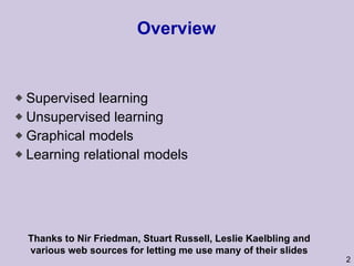
This document provides an overview and introduction to machine learning and probabilistic graphical models. It discusses key topics such as supervised learning, unsupervised learning, graphical models, inference, and structure learning. The document covers techniques like decision trees, neural networks, clustering, dimensionality reduction, Bayesian networks, and learning the structure of probabilistic graphical models.

1. An introduction to machine learning and probabilistic graphical models Kevin Murphy MIT AI Lab Presented at Intel’s workshop on “Machine learning for the life sciences”, Berkeley, CA, 3 November 2003

2. Overview Supervised learning Unsupervised learning Graphical models Learning relational models Thanks to Nir Friedman, Stuart Russell, Leslie Kaelbling and various web sources for letting me use many of their slides

3. Supervised learning yes no N Small Arrow Red Y Small Star Blue Y Small Square Blue Y Big Torus Blue Output Size Shape Color F(x1, x2, x3) -> t Learn to approximate function from a training set of (x,t) pairs

4. Supervised learning Learner Training data Hypothesis Testing data Prediction N S A R Y S S B Y S S B Y B T B T X3 X2 X1 ? S C Y ? S A B T X3 X2 X1 N Y T

5. Key issue: generalization yes no ? ? Can’t just memorize the training set (overfitting)

6. Hypothesis spaces Decision trees Neural networks K-nearest neighbors Naïve Bayes classifier Support vector machines (SVMs) Boosted decision stumps …

7. Perceptron (neural net with no hidden layers) Linearly separable data

8. Which separating hyperplane?

9. The linear separator with the largest margin is the best one to pick margin

10. What if the data is not linearly separable?

11. Kernel trick kernel Kernel implicitly maps from 2D to 3D, making problem linearly separable x 1 x 2 z 1 z 2 z 3

12. Support Vector Machines (SVMs) Two key ideas: Large margins Kernel trick

13. Boosting Simple classifiers (weak learners) can have their performance boosted by taking weighted combinations Boosting maximizes the margin

14. Supervised learning success stories Face detection Steering an autonomous car across the US Detecting credit card fraud Medical diagnosis …

15. Unsupervised learning What if there are no output labels?

16. K-means clustering Guess number of clusters, K Guess initial cluster centers,  1 ,  2 Assign data points x i to nearest cluster center Re-compute cluster centers based on assignments Reiterate

17. AutoClass (Cheeseman et al, 1986) EM algorithm for mixtures of Gaussians “ Soft” version of K-means Uses Bayesian criterion to select K Discovered new types of stars from spectral data Discovered new classes of proteins and introns from DNA/protein sequence databases

18. Hierarchical clustering

19. Principal Component Analysis (PCA) PCA seeks a projection that best represents the data in a least-squares sense. PCA reduces the dimensionality of feature space by restricting attention to those directions along which the scatter of the cloud is greatest.

20. Discovering nonlinear manifolds

21. Combining supervised and unsupervised learning

22. Discovering rules (data mining) Find the most frequent patterns (association rules) Num in household = 1 ^ num children = 0 => language = English Language = English ^ Income < $40k ^ Married = false ^ num children = 0 => education {college, grad school} HS MD PhD MA Educ. $30k $80k $20k $10k Income Retired Doctor Student Student Occup. 60 M F 30 M M 24 S F 22 S M Age Married Sex

23. Unsupervised learning: summary Clustering Hierarchical clustering Linear dimensionality reduction (PCA) Non-linear dim. Reduction Learning rules

24. Discovering networks ? From data visualization to causal discovery

25. Networks in biology Most processes in the cell are controlled by networks of interacting molecules: Metabolic Network Signal Transduction Networks Regulatory Networks Networks can be modeled at multiple levels of detail/ realism Molecular level Concentration level Qualitative level Decreasing detail

26. Molecular level: Lysis-Lysogeny circuit in Lambda phage Arkin et al. (1998), Genetics 149(4):1633-48 5 genes, 67 parameters based on 50 years of research Stochastic simulation required supercomputer

27. Concentration level: metabolic pathways Usually modeled with differential equations w 23 g1 g2 g3 g4 g5 w 12 w 55

28. Qualitative level: Boolean Networks

29. Probabilistic graphical models Supports graph-based modeling at various levels of detail Models can be learned from noisy, partial data Can model “inherently” stochastic phenomena, e.g., molecular-level fluctuations… But can also model deterministic, causal processes. &quot;The actual science of logic is conversant at present only with things either certain, impossible, or entirely doubtful. Therefore the true logic for this world is the calculus of probabilities.&quot; -- James Clerk Maxwell &quot;Probability theory is nothing but common sense reduced to calculation.&quot; -- Pierre Simon Laplace

30. Graphical models: outline What are graphical models? Inference Structure learning

31. Simple probabilistic model: linear regression Y Y =  +  X + noise Deterministic (functional) relationship X

32. Simple probabilistic model: linear regression Y Y =  +  X + noise Deterministic (functional) relationship X “ Learning” = estimating parameters  ,  ,  from (x,y) pairs. Can be estimate by least squares Is the empirical mean Is the residual variance

33. Piecewise linear regression Latent “switch” variable – hidden process at work

34. Probabilistic graphical model for piecewise linear regression Hidden variable Q chooses which set of parameters to use for predicting Y. Value of Q depends on value of input X. output input This is an example of “mixtures of experts” Learning is harder because Q is hidden, so we don’t know which data points to assign to each line; can be solved with EM (c.f., K-means) X Y Q

35. Classes of graphical models Probabilistic models Graphical models Directed Undirected Bayes nets MRFs DBNs

36. Bayesian Networks Qualitative part : Directed acyclic graph (DAG) Nodes - random variables Edges - direct influence Quantitative part : Set of conditional probability distributions Earthquake Radio Burglary Alarm Call Compact representation of probability distributions via conditional independence Together: Define a unique distribution in a factored form Family of Alarm 0.9 0.1 e b e 0.2 0.8 0.01 0.99 0.9 0.1 b e b b e B E P(A | E,B)

37. Example: “ICU Alarm” network Domain: Monitoring Intensive-Care Patients 37 variables 509 parameters …instead of 2 54 PCWP CO HRBP HREKG HRSAT ERRCAUTER HR HISTORY CATECHOL SAO2 EXPCO2 ARTCO2 VENTALV VENTLUNG VENITUBE DISCONNECT MINVOLSET VENTMACH KINKEDTUBE INTUBATION PULMEMBOLUS PAP SHUNT ANAPHYLAXIS MINOVL PVSAT FIO2 PRESS INSUFFANESTH TPR LVFAILURE ERRBLOWOUTPUT STROEVOLUME LVEDVOLUME HYPOVOLEMIA CVP BP

38. Success stories for graphical models Multiple sequence alignment Forensic analysis Medical and fault diagnosis Speech recognition Visual tracking Channel coding at Shannon limit Genetic pedigree analysis …

39. Graphical models: outline What are graphical models? p Inference Structure learning

40. Probabilistic Inference Posterior probabilities Probability of any event given any evidence P(X|E) Radio Call Earthquake Radio Burglary Alarm Call

41. Viterbi decoding Y 1 Y 3 X 1 X 2 X 3 Y 2 Compute most probable explanation (MPE) of observed data Hidden Markov Model (HMM) “ Tomato” hidden observed

42. Inference: computational issues Easy Hard Chains Trees Grids Dense, loopy graphs PCWP CO HRBP HREKG HRSAT ERRCAUTER HR HISTORY CATECHOL SAO2 EXPCO2 ARTCO2 VENTALV VENTLUNG VENITUBE DISCONNECT MINVOLSET VENTMACH KINKEDTUBE INTUBATION PULMEMBOLUS PAP SHUNT MINOVL PVSAT PRESS INSUFFANESTH TPR LVFAILURE ERRBLOWOUTPUT STROEVOLUME LVEDVOLUME HYPOVOLEMIA CVP BP

43. Inference: computational issues Easy Hard Chains Trees Grids Dense, loopy graphs Many difference inference algorithms, both exact and approximate PCWP CO HRBP HREKG HRSAT ERRCAUTER HR HISTORY CATECHOL SAO2 EXPCO2 ARTCO2 VENTALV VENTLUNG VENITUBE DISCONNECT MINVOLSET VENTMACH KINKEDTUBE INTUBATION PULMEMBOLUS PAP SHUNT MINOVL PVSAT PRESS INSUFFANESTH TPR LVFAILURE ERRBLOWOUTPUT STROEVOLUME LVEDVOLUME HYPOVOLEMIA CVP BP

44. Bayesian inference Bayesian probability treats parameters as random variables Learning/ parameter estimation is replaced by probabilistic inference P(  |D) Example: Bayesian linear regression; parameters are  = (  ,  ,  )  X 1 Y 1 X n Y n Parameters are tied (shared) across repetitions of the data

45. Bayesian inference + Elegant – no distinction between parameters and other hidden variables + Can use priors to learn from small data sets (c.f., one-shot learning by humans) - Math can get hairy - Often computationally intractable

46. Graphical models: outline What are graphical models? Inference Structure learning p p

47. Why Struggle for Accurate Structure? Increases the number of parameters to be estimated Wrong assumptions about domain structure Cannot be compensated for by fitting parameters Wrong assumptions about domain structure Adding an arc Missing an arc Earthquake Alarm Set Sound Burglary Earthquake Alarm Set Sound Burglary Earthquake Alarm Set Sound Burglary Truth

48. Score ­b ased Learning E B A E B A E B A Search for a structure that maximizes the score Define scoring function that evaluates how well a structure matches the data E, B, A <Y,N,N> <Y,Y,Y> <N,N,Y> <N,Y,Y> . . <N,Y,Y>

49. Learning Trees Can find optimal tree structure in O(n 2 log n) time: just find the max-weight spanning tree If some of the variables are hidden, problem becomes hard again, but can use EM to fit mixtures of trees

50. Heuristic Search Learning arbitrary graph structure is NP-hard. So it is common to resort to heuristic search Define a search space: search states are possible structures operators make small changes to structure Traverse space looking for high-scoring structures Search techniques: Greedy hill-climbing Best first search Simulated Annealing ...

51. Local Search Operations Typical operations: Reverse C  E Delete C  E Add C  D  score = S({C,E}  D) - S({E}  D) S C E D S C E D S C E D S C E D

52. Problems with local search S(G|D) Easy to get stuck in local optima “ truth” you

53. Problems with local search II Picking a single best model can be misleading E R B A C P(G|D)

54. Problems with local search II Small sample size  many high scoring models Answer based on one model often useless Want features common to many models Picking a single best model can be misleading E R B A C E R B A C E R B A C E R B A C E R B A C P(G|D)

55. Bayesian Approach to Structure Learning Posterior distribution over structures Estimate probability of features Edge X  Y Path X  …  Y … Feature of G , e.g., X  Y Indicator function for feature f Bayesian score for G

56. Bayesian approach: computational issues Posterior distribution over structures How compute sum over super-exponential number of graphs? MCMC over networks MCMC over node-orderings (Rao-Blackwellisation)

57. Structure learning: other issues Discovering latent variables Learning causal models Learning from interventional data Active learning

58. Discovering latent variables a) 17 parameters b) 59 parameters There are some techniques for automatically detecting the possible presence of latent variables

59. Learning causal models So far, we have only assumed that X -> Y -> Z means that Z is independent of X given Y. However, we often want to interpret directed arrows causally. This is uncontroversial for the arrow of time. But can we infer causality from static observational data?

60. Learning causal models We can infer causality from static observational data if we have at least four measured variables and certain “tetrad” conditions hold. See books by Pearl and Spirtes et al. However, we can only learn up to Markov equivalence, not matter how much data we have. X Y Z X Y Z X Y Z X Y Z

61. Learning from interventional data The only way to distinguish between Markov equivalent networks is to perform interventions, e.g., gene knockouts. We need to (slightly) modify our learning algorithms. smoking Yellow fingers P(smoker|observe(yellow)) >> prior smoking Yellow fingers P(smoker | do(paint yellow)) = prior Cut arcs coming into nodes which were set by intervention

62. Active learning Which experiments (interventions) should we perform to learn structure as efficiently as possible? This problem can be modeled using decision theory. Exact solutions are wildly computationally intractable. Can we come up with good approximate decision making techniques? Can we implement hardware to automatically perform the experiments? “AB: Automated Biologist”

63. Learning from relational data Can we learn concepts from a set of relations between objects, instead of/ in addition to just their attributes?

64. Learning from relational data: approaches Probabilistic relational models (PRMs) Reify a relationship (arcs) between nodes (objects) by making into a node (hypergraph) Inductive Logic Programming (ILP) Top-down, e.g., FOIL (generalization of C4.5) Bottom up, e.g., PROGOL (inverse deduction)

65. ILP for learning protein folding: input yes no TotalLength(D2mhr, 118) ^ NumberHelices(D2mhr, 6) ^ … 100 conjuncts describing structure of each pos/neg example

66. ILP for learning protein folding: results PROGOL learned the following rule to predict if a protein will form a “four-helical up-and-down bundle”: In English: “The protein P folds if it contains a long helix h 1 at a secondary structure position between 1 and 3 and h 1 is next to a second helix”

67. ILP: Pros and Cons + Can discover new predicates (concepts) automatically + Can learn relational models from relational (or flat) data - Computationally intractable - Poor handling of noise

68. The future of machine learning for bioinformatics? Oracle

69. The future of machine learning for bioinformatics Learner Prior knowledge Replicated experiments Biological literature Hypotheses Expt. design Real world “ Computer assisted pathway refinement”

70. The end

71. Decision trees blue? big? oval? no no yes yes

72. Decision trees blue? big? oval? no no yes yes + Handles mixed variables + Handles missing data + Efficient for large data sets + Handles irrelevant attributes + Easy to understand - Predictive power

73. Feedforward neural network input Hidden layer Output Weights on each arc Sigmoid function at each node

74. Feedforward neural network input Hidden layer Output - Handles mixed variables - Handles missing data - Efficient for large data sets - Handles irrelevant attributes - Easy to understand + Predicts poorly

75. Nearest Neighbor Remember all your data When someone asks a question, find the nearest old data point return the answer associated with it

76. Nearest Neighbor ? - Handles mixed variables - Handles missing data - Efficient for large data sets - Handles irrelevant attributes - Easy to understand + Predictive power

77. Support Vector Machines (SVMs) Two key ideas: Large margins are good Kernel trick

78. SVM: mathematical details Training data : l -dimensional vector with flag of true or false Separating hyperplane : Inequalities : Margin : Support vectors : Support vector expansion: Decision: margin

79. Replace all inner products with kernels Kernel function

80. SVMs: summary - Handles mixed variables - Handles missing data - Efficient for large data sets - Handles irrelevant attributes - Easy to understand + Predictive power Kernel trick can be used to make many linear methods non-linear e.g., kernel PCA, kernelized mutual information Large margin classifiers are good General lessons from SVM success:

81. Boosting: summary Can boost any weak learner Most commonly: boosted decision “stumps” + Handles mixed variables + Handles missing data + Efficient for large data sets + Handles irrelevant attributes - Easy to understand + Predictive power

82. Supervised learning: summary Learn mapping F from inputs to outputs using a training set of (x,t) pairs F can be drawn from different hypothesis spaces, e.g., decision trees, linear separators, linear in high dimensions, mixtures of linear Algorithms offer a variety of tradeoffs Many good books, e.g., “ The elements of statistical learning”, Hastie, Tibshirani, Friedman, 2001 “ Pattern classification”, Duda, Hart, Stork, 2001

83. Inference Posterior probabilities Probability of any event given any evidence Most likely explanation Scenario that explains evidence Rational decision making Maximize expected utility Value of Information Effect of intervention Radio Call Earthquake Radio Burglary Alarm Call

84. Assumption needed to make learning work We need to assume “Future futures will resemble past futures” (B. Russell) Unlearnable hypothesis: “All emeralds are grue”, where “grue” means: green if observed before time t, blue afterwards.

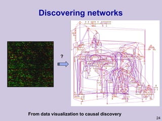
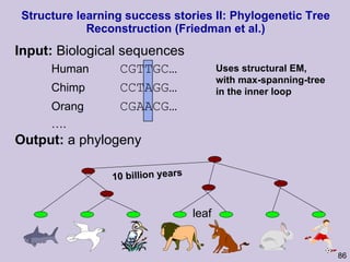
85. Structure learning success stories: gene regulation network (Friedman et al.) Yeast data [Hughes et al 2000] 600 genes 300 experiments

86. Structure learning success stories II: Phylogenetic Tree Reconstruction (Friedman et al.) Input: Biological sequences Human CGTTGC… Chimp CCTAGG… Orang CGAACG… … . Output: a phylogeny 10 billion years Uses structural EM, with max-spanning-tree in the inner loop leaf

87. Instances of graphical models Probabilistic models Graphical models Directed Undirected Bayes nets MRFs DBNs Hidden Markov Model (HMM) Naïve Bayes classifier Mixtures of experts Kalman filter model Ising model

88. ML enabling technologies Faster computers More data The web Parallel corpora (machine translation) Multiple sequenced genomes Gene expression arrays New ideas Kernel trick Large margins Boosting Graphical models …