This document discusses probabilistic modeling and decision theory. It describes how probabilistic models can be used to make decisions based on observed data and prior knowledge. The key aspects covered include:
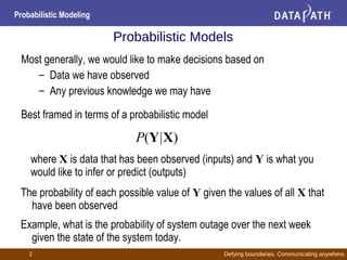
- Probabilistic models express the probability of outcomes given observed data.
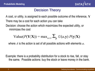
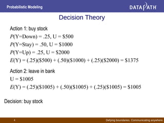
- Decision theory involves assigning costs to outcomes and choosing the action that maximizes expected utility.
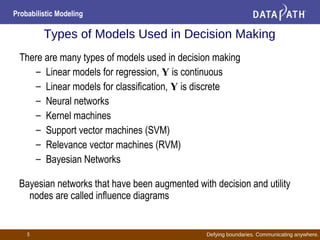
- Common probabilistic models for decision making include Bayesian networks, neural networks, and support vector machines.
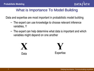
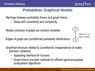
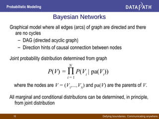
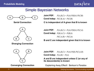
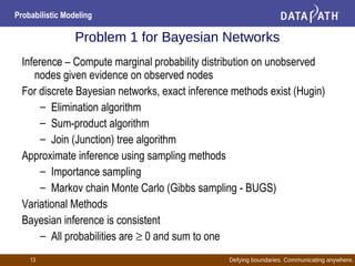
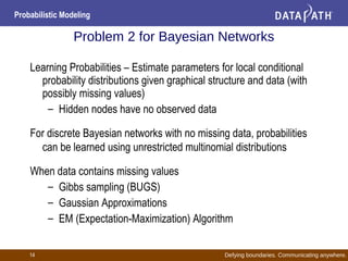
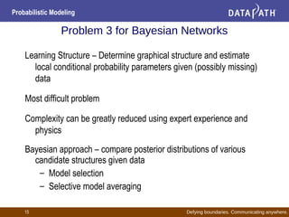
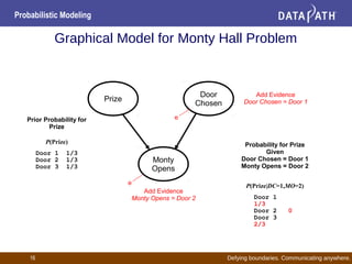
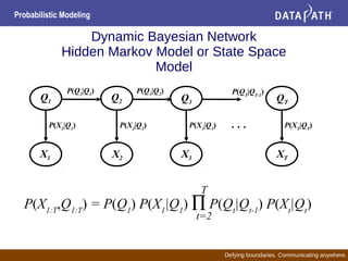
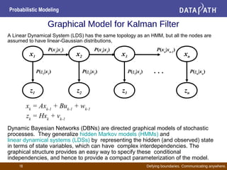
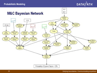
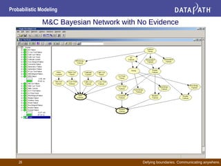
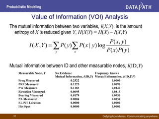
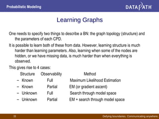
- Bayesian networks represent conditional dependencies graphically and can be used for inference, parameter estimation, and structure learning.