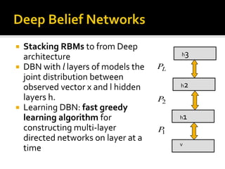
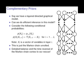
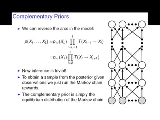
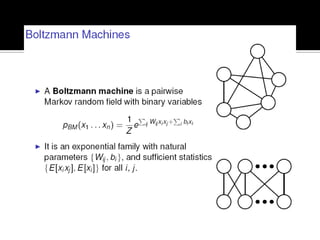
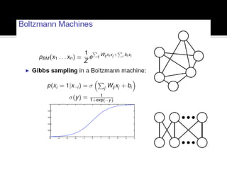
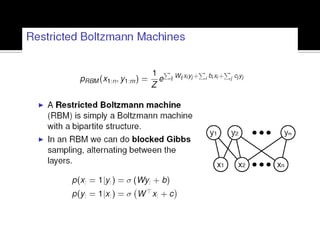
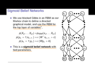
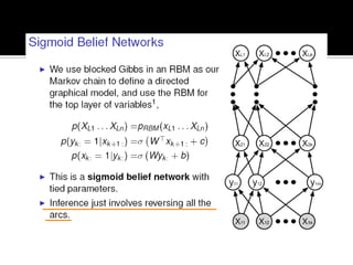
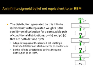
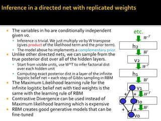
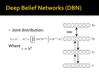
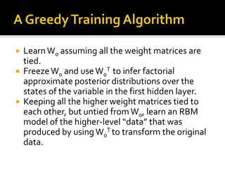
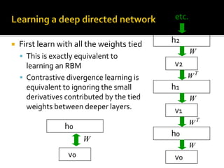
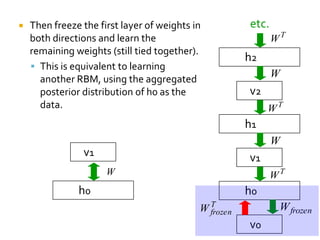
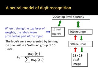
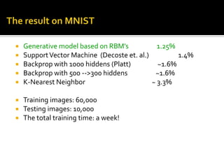
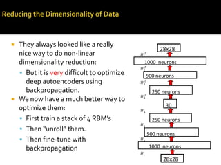
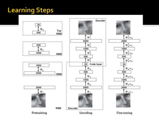
CS590M 2008 Fall: Paper PresentationDeep Belief Nets Presenters:Sael Lee, Rongjing Xiang, SuleymanCetintas, Youhan FangDepartment of Computer Science, Purdue UniversityMajor reference paper: Hinton, G. E, Osindero, S., and Teh, Y. W. (2006). A fast learning algorithm for deep belief nets. Neural Computation, 18:1527-1554
OutlineIntroduction Complementary priorRestricted Boltzmann machinesDeep Belief networksApplications Papers
What is Deep Belief Network(DBN)?  h3DBNs are stacks of restricted Boltzmann machines forming deep (multi-layer) architecture. 2000 top-level neuronsRBM500 neuronsh2RBM500 neurons        h1   28x28 pixel image (784 neurons)RBM   data
Deep NetworksWhy go deep??Insufficient depth can require more computational elements,  than architectures whose depth is matches to the task. Provide simpler more descriptive model of many problems.Problem with deep?Many cases, deep nets are hard to optimize. Deep Networks     		Neural 	               NetworksDeep Belief Nets.
Belief Nets (Bayesian Network) Stochastic hidden causeA belief net is a directed acyclic graph composed of stochastic variables.It is easy to generate an unbiased samples at the leaf nodes, so we can see what kinds of data the network believes in.It is hard to infer the posterior distribution over all  possible configurations of hidden causes. (explaining away effect)It is hard to even get  a sample from the posterior.So how can we learn deep belief nets that have millions of parameters? -> use Restrictive Boltzmann machines for each layer!! visible  effectWe will use nets composed of layers of stochastic binary variables with weighted connections
Why it is usually very hard to learn belief nets one layer at a timeTo learn W, we need the posterior distribution in the first hidden layer.Problem 1: The posterior is typically intractable because of “explaining away”.Problem 2: The posterior depends on the prior as well as the likelihood. So to learn W, we need to know the weights in higher layers, even if we are only approximating the posterior. All the weights interact.Problem 3: We need to integrate over all possible configurations of the higher variables to get the prior for first hidden layer. hidden variableshidden variablespriorhidden variablesW  likelihood          data
Energy-Based ModelsDeep Belief nets are composed of Restricted Boltzmann machines which are energy based models     Energy based modelsdefine probability distribution through an energy function: Data log likelihood gradient“f” is the expert
Boltzmann machinesOne type of Generative Neural network that connect binary stochastic neurons using symmetric connections. b and c are bias of x and h, W,U,V are weights
Restricted Boltzmann machines (RBM)binary state of visible unit ihiddenbinary state of hidden unit jWe restrict the connectivity to make learning easier.Only one layer of hidden units.We will deal with more layers laterNo connections between hidden units.In an RBM, the hidden units are conditionally independent given the visible states.  So we can quickly get an unbiased sample from the posterior distribution when given a data-vector.This is a big advantage over directed belief netsApproximation of the log-likelihood gradient: Contrastive DivergencejivisibleEnergy with configuration v on the visible units and h on the hidden unitsweight between units i and j
Deep Belief Networksh3Stacking RBMs to from Deep architectureDBN with l layers of models the joint distribution between observed vector x and l hidden layers h. Learning DBN: fast greedy learning algorithm for constructing multi-layer directed networks on layer at a time      h2     h1     v
Inference in Directed Belief Networks: Why Hard?Explaining AwayPosterior over Hidden Vars. <-> intractableVariational Methods approximate the true posterior and improve a lower bound on the log probability of the training datathis works, but there is a better alternative:Eliminating Explaining Away in Logistic (Sigmoid) Belief NetsPosterior(non-indep) = prior(indep.) * likelihood (non-indep.)Eliminate Explaining Away by Complementary PriorsAdd extra hidden layers to create CP that has opposite correlations with the likelihood term, so (when likelihood is multiplied by the prior), post. will become factorial
An infinite sigmoid belief net equivalent to an RBMetc.         h2The distribution generated by this infinite directed net with replicated weights is the equilibrium distribution for a compatible pair of conditional distributions: p(v|h) and p(h|v) that are both defined by WA top-down pass of the directed net = letting a Restricted Boltzmann Machine settle to equilibrium.So this infinite directed net  defines the same distribution as an RBM.    v2         h1    v1         h0    v0
Inference in a directed net with replicated weightsetc.The variables in h0 are conditionally independent given v0.Inference is trivial. We just multiply v0 by W transpose (gives product of the likelihood term and the prior term).The model above h0 implements a complementary prior.Unlike other directed nets, we can sample from the true posterior dist over all of the hidden layers.Start from visible units, use W^T to infer factorial dist over each hidden unitComputing exact posterior dist in a layer of the infinite logistic belief net = each step of Gibbs sampling in RBMThe Maximum Likelihood learning rule for the infinite logistic belief net with tied weights is the same with the learning rule of RBMContrastive Divergence can be used instead of Maximum likelihood learning which is expensiveRBM creates good generative models that can be fine-tuned         h2    v2         h1      v1++            h0++    v0
Deep Belief Networks (DBN)Joint distribution:Where
A Greedy Training AlgorithmLearn W0assuming all the weight matrices are tied. Freeze W0and use W0Tto infer factorial approximate posterior distributions over the states of the variable in the first hidden layer.Keeping all the higher weight matrices tied to each other, but untied from W0, learn an RBM model of the higher-level “data” that was produced by using W0T to transform the original data.
Learning a deep directed networketc.         h2First learn with all the weights tied
This is exactly equivalent to learning an RBM
Contrastive divergence learning is equivalent to ignoring the small derivatives contributed by the tied weights between deeper layers.    v2         h1    v1         h0         h0    v0    v0
etc.Then freeze the first layer of weights in both directions and learn the remaining weights (still tied together).This is equivalent to learning another RBM, using the aggregated posterior distribution of h0 as the data.         h2    v2         h1    v1    v1         h0         h0    v0
What happens when the weights in higher layers become different from the weights in the first layer?The higher layers no longer implement a complementary prior.So performing inference using the frozen weights in the first layer is no longer correct. Using this incorrect inference procedure gives a variational  lower bound on the log probability of the data. We lose by the slackness of the bound.The higher layers learn a prior that is closer to the aggregated posterior distribution of the first hidden layer.This improves the network’s model of the data.Hinton, Osindero and Teh (2006) prove that this improvement is always bigger than the loss.
Fine-tuning with a contrastive divergence version of the “wake-sleep” algorithmAfter learning many layers of features, we can fine-tune the features to improve generation.
1. Do a stochastic bottom-up pass
Adjust the top-down weights to be good at reconstructing the feature activities in the layer below.
2. Do a few iterations of sampling in the top level RBM
Use CD learning to improve the RBM
3. Do a stochastic top-down pass
Adjust the bottom-up weights to be good at reconstructing the feature activities in the layer above.A neural model of digit recognition2000 top-level neuronsWhen training the top layer of weights, the labels were provided as part of the input10 label neurons500 neuronsThe labels were represented by turning on one unit in a ‘softmax’ group of 10 units:500 neurons28 x 28 pixel     image
The result on MNISTGenerative model based on RBM’s                   1.25%Support Vector Machine  (Decoste et. al.)	      1.4%   Backprop with 1000 hiddens (Platt)                  ~1.6%Backprop with 500 -->300 hiddens                   ~1.6%K-Nearest Neighbor                                             ~ 3.3%Training images: 60,000Testing images: 10,000The total training time: a week!
Looking into the ‘mind’ of the machineSamples generated by letting the associative memory run with one label clamped.
Looking into the ‘mind’ of the machineProviding a random binary image as input

Deep Belief nets

  • 1.
    CS590M 2008 Fall:Paper PresentationDeep Belief Nets Presenters:Sael Lee, Rongjing Xiang, SuleymanCetintas, Youhan FangDepartment of Computer Science, Purdue UniversityMajor reference paper: Hinton, G. E, Osindero, S., and Teh, Y. W. (2006). A fast learning algorithm for deep belief nets. Neural Computation, 18:1527-1554
  • 2.
    OutlineIntroduction Complementary priorRestrictedBoltzmann machinesDeep Belief networksApplications Papers
  • 3.
    What is DeepBelief Network(DBN)? h3DBNs are stacks of restricted Boltzmann machines forming deep (multi-layer) architecture. 2000 top-level neuronsRBM500 neuronsh2RBM500 neurons h1 28x28 pixel image (784 neurons)RBM data
  • 4.
    Deep NetworksWhy godeep??Insufficient depth can require more computational elements, than architectures whose depth is matches to the task. Provide simpler more descriptive model of many problems.Problem with deep?Many cases, deep nets are hard to optimize. Deep Networks Neural NetworksDeep Belief Nets.
  • 5.
    Belief Nets (BayesianNetwork) Stochastic hidden causeA belief net is a directed acyclic graph composed of stochastic variables.It is easy to generate an unbiased samples at the leaf nodes, so we can see what kinds of data the network believes in.It is hard to infer the posterior distribution over all possible configurations of hidden causes. (explaining away effect)It is hard to even get a sample from the posterior.So how can we learn deep belief nets that have millions of parameters? -> use Restrictive Boltzmann machines for each layer!! visible effectWe will use nets composed of layers of stochastic binary variables with weighted connections
  • 6.
    Why it isusually very hard to learn belief nets one layer at a timeTo learn W, we need the posterior distribution in the first hidden layer.Problem 1: The posterior is typically intractable because of “explaining away”.Problem 2: The posterior depends on the prior as well as the likelihood. So to learn W, we need to know the weights in higher layers, even if we are only approximating the posterior. All the weights interact.Problem 3: We need to integrate over all possible configurations of the higher variables to get the prior for first hidden layer. hidden variableshidden variablespriorhidden variablesW likelihood data
  • 7.
    Energy-Based ModelsDeep Beliefnets are composed of Restricted Boltzmann machines which are energy based models Energy based modelsdefine probability distribution through an energy function: Data log likelihood gradient“f” is the expert
  • 8.
    Boltzmann machinesOne typeof Generative Neural network that connect binary stochastic neurons using symmetric connections. b and c are bias of x and h, W,U,V are weights
  • 9.
    Restricted Boltzmann machines(RBM)binary state of visible unit ihiddenbinary state of hidden unit jWe restrict the connectivity to make learning easier.Only one layer of hidden units.We will deal with more layers laterNo connections between hidden units.In an RBM, the hidden units are conditionally independent given the visible states. So we can quickly get an unbiased sample from the posterior distribution when given a data-vector.This is a big advantage over directed belief netsApproximation of the log-likelihood gradient: Contrastive DivergencejivisibleEnergy with configuration v on the visible units and h on the hidden unitsweight between units i and j
  • 10.
    Deep Belief Networksh3StackingRBMs to from Deep architectureDBN with l layers of models the joint distribution between observed vector x and l hidden layers h. Learning DBN: fast greedy learning algorithm for constructing multi-layer directed networks on layer at a time h2 h1 v
  • 11.
    Inference in DirectedBelief Networks: Why Hard?Explaining AwayPosterior over Hidden Vars. <-> intractableVariational Methods approximate the true posterior and improve a lower bound on the log probability of the training datathis works, but there is a better alternative:Eliminating Explaining Away in Logistic (Sigmoid) Belief NetsPosterior(non-indep) = prior(indep.) * likelihood (non-indep.)Eliminate Explaining Away by Complementary PriorsAdd extra hidden layers to create CP that has opposite correlations with the likelihood term, so (when likelihood is multiplied by the prior), post. will become factorial
  • 22.
    An infinite sigmoidbelief net equivalent to an RBMetc. h2The distribution generated by this infinite directed net with replicated weights is the equilibrium distribution for a compatible pair of conditional distributions: p(v|h) and p(h|v) that are both defined by WA top-down pass of the directed net = letting a Restricted Boltzmann Machine settle to equilibrium.So this infinite directed net defines the same distribution as an RBM. v2 h1 v1 h0 v0
  • 23.
    Inference in adirected net with replicated weightsetc.The variables in h0 are conditionally independent given v0.Inference is trivial. We just multiply v0 by W transpose (gives product of the likelihood term and the prior term).The model above h0 implements a complementary prior.Unlike other directed nets, we can sample from the true posterior dist over all of the hidden layers.Start from visible units, use W^T to infer factorial dist over each hidden unitComputing exact posterior dist in a layer of the infinite logistic belief net = each step of Gibbs sampling in RBMThe Maximum Likelihood learning rule for the infinite logistic belief net with tied weights is the same with the learning rule of RBMContrastive Divergence can be used instead of Maximum likelihood learning which is expensiveRBM creates good generative models that can be fine-tuned h2 v2 h1 v1++ h0++ v0
  • 24.
    Deep Belief Networks(DBN)Joint distribution:Where
  • 25.
    A Greedy TrainingAlgorithmLearn W0assuming all the weight matrices are tied. Freeze W0and use W0Tto infer factorial approximate posterior distributions over the states of the variable in the first hidden layer.Keeping all the higher weight matrices tied to each other, but untied from W0, learn an RBM model of the higher-level “data” that was produced by using W0T to transform the original data.
  • 26.
    Learning a deepdirected networketc. h2First learn with all the weights tied
  • 27.
    This is exactlyequivalent to learning an RBM
  • 28.
    Contrastive divergence learningis equivalent to ignoring the small derivatives contributed by the tied weights between deeper layers. v2 h1 v1 h0 h0 v0 v0
  • 29.
    etc.Then freeze thefirst layer of weights in both directions and learn the remaining weights (still tied together).This is equivalent to learning another RBM, using the aggregated posterior distribution of h0 as the data. h2 v2 h1 v1 v1 h0 h0 v0
  • 30.
    What happens whenthe weights in higher layers become different from the weights in the first layer?The higher layers no longer implement a complementary prior.So performing inference using the frozen weights in the first layer is no longer correct. Using this incorrect inference procedure gives a variational lower bound on the log probability of the data. We lose by the slackness of the bound.The higher layers learn a prior that is closer to the aggregated posterior distribution of the first hidden layer.This improves the network’s model of the data.Hinton, Osindero and Teh (2006) prove that this improvement is always bigger than the loss.
  • 31.
    Fine-tuning with acontrastive divergence version of the “wake-sleep” algorithmAfter learning many layers of features, we can fine-tune the features to improve generation.
  • 32.
    1. Do astochastic bottom-up pass
  • 33.
    Adjust the top-downweights to be good at reconstructing the feature activities in the layer below.
  • 34.
    2. Do afew iterations of sampling in the top level RBM
  • 35.
    Use CD learningto improve the RBM
  • 36.
    3. Do astochastic top-down pass
  • 37.
    Adjust the bottom-upweights to be good at reconstructing the feature activities in the layer above.A neural model of digit recognition2000 top-level neuronsWhen training the top layer of weights, the labels were provided as part of the input10 label neurons500 neuronsThe labels were represented by turning on one unit in a ‘softmax’ group of 10 units:500 neurons28 x 28 pixel image
  • 38.
    The result onMNISTGenerative model based on RBM’s 1.25%Support Vector Machine (Decoste et. al.) 1.4% Backprop with 1000 hiddens (Platt) ~1.6%Backprop with 500 -->300 hiddens ~1.6%K-Nearest Neighbor ~ 3.3%Training images: 60,000Testing images: 10,000The total training time: a week!
  • 39.
    Looking into the‘mind’ of the machineSamples generated by letting the associative memory run with one label clamped.
  • 40.
    Looking into the‘mind’ of the machineProviding a random binary image as input