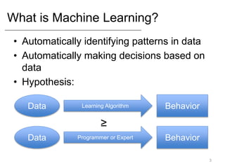
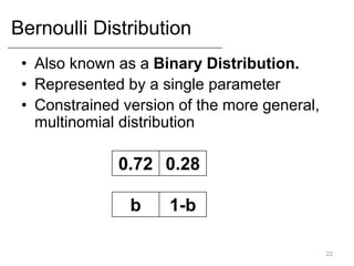
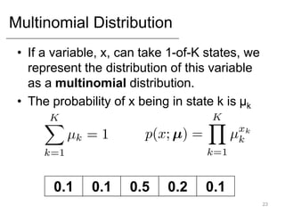
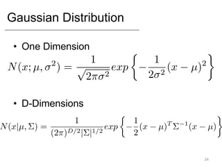
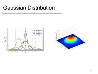
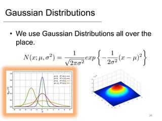
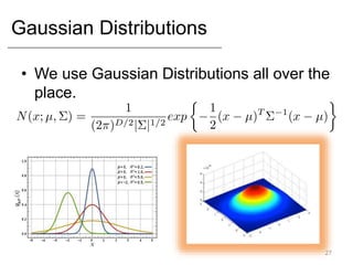
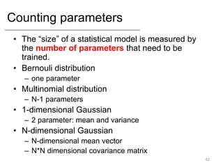
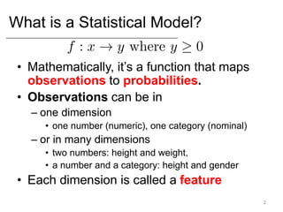
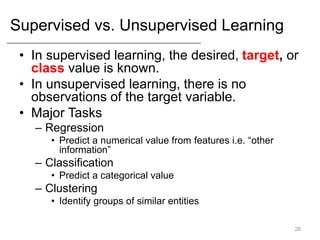
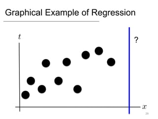
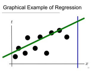
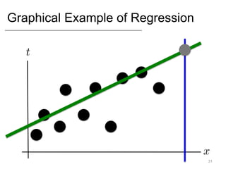
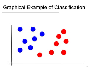
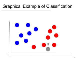
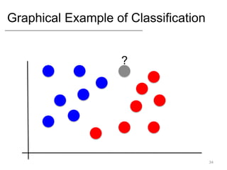
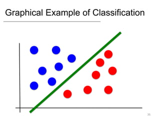
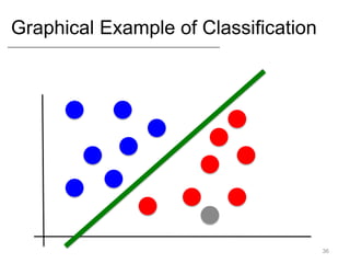
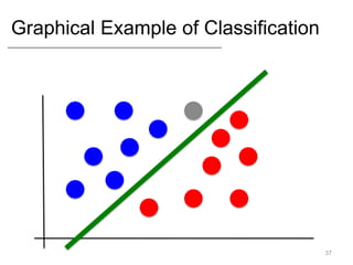
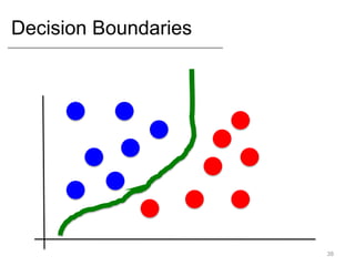
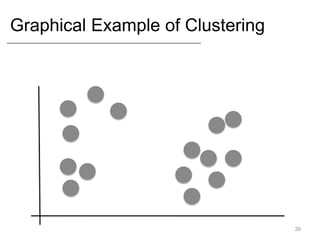
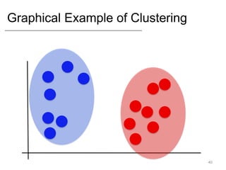
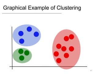
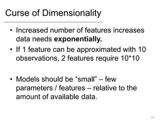
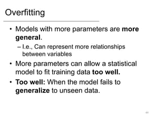
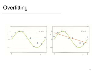
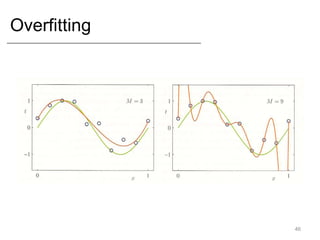
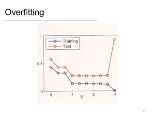
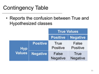
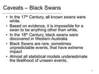
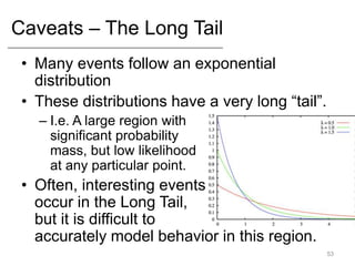
This document provides an introduction to statistical modeling and machine learning concepts. It discusses: - What statistical modeling and machine learning are, including training models on data and evaluating them. - Common statistical models like Gaussian, Bernoulli, and Multinomial distributions. - Supervised learning tasks like regression and classification, and unsupervised clustering. - Key concepts like overfitting, evaluation metrics, and issues with modeling like black swans and the long tail.

1. Introduction to Statistical
Modeling and Machine
Learning
Lecture 8
Spoken Language Processing
Prof. Andrew Rosenberg

2. What is Statistical Modeling
• Statistical Modeling is the process of using
data to construct a mathematical or
algorithmic device to measure the probability
of some observation.
• Training
– Using a set of observations to learn parameters
of a model, or construct the decision making
process.
• Evaluation
– Determining the probability of a new observation
1

3. What is a Statistical Model?
• Mathematically, it’s a function that maps
observations to probabilities.
• Observations can be in
– one dimension
• one number (numeric), one category (nominal)
– or in many dimensions
• two numbers: height and weight,
• a number and a category: height and gender
• Each dimension is called a feature
2

4. What is Machine Learning?
• Automatically identifying patterns in data
• Automatically making decisions based on
data
• Hypothesis:
3
Data Learning Algorithm Behavior
Data Programmer or Expert Behavior
≥

5. Basics of Probabilities.
• Probabilities fall in the range [0,1]
• Mutually Exclusive events are events
that cannot simultaneously occur.
– The sum of the likelihoods of all mutually
exclusive events must be 1.
4

6. Joint Probability
• We can represent the probability of more
than one event at the same time.
• If two events are independent.
5

7. Joint Probability Table
6
• A Joint Probability function defines the likelihood of two
(or more) events occurring.
• Let nij be the number of times event i and event j
simultaneously occur.
Orange Green
Blue box 1 3 4
Red box 6 2 8
7 5 12

8. Marginalization
7
• Consider the probability of X irrespective of Y.
• The number of instances in column j is the sum of
instances in each cell
• Therefore, we can marginalize or “sum over” Y:

9. Conditional Probability
8
• Consider only instances where X = xj.
• The fraction of these instances where Y =
yi is the conditional probability
– “The probability of y given x”

10. Relating the Joint Conditional and
Marginal
9

11. Sum and Product Rules
• In general, we’ll refer to a distribution over
a random variable as p(X) and a
distribution evaluated at a particular value
as p(x).
10
Sum Rule
Product Rule

12. Bayes Rule
11

13. Interpretation of Bayes Rule
12
• Prior: Information we have before
observation.
• Posterior: The distribution of Y after
observing X
• Likelihood: The likelihood of observing X
given Y
Prior
Posterior
Likelihood

14. Expected Values
• The expected value of a random variable is a
weighted average.
• Expected values
are used to
determine what is
likely to happen
in a random setting
• Expectation
– The expected value of a function is the hypothesis
• Variance
– The variance is the confidence in that hypothesis
13

15. What is a Probability?
• Frequentists
– A probability is the likelihood that an event
will happen
– It is approximated by the ratio of the number
of observed events to the number of total
events
– Assessment is vital to selecting a model
– Point estimates are absolutely fine
14

16. What is a Probability?
• Bayesians
– A probability is a degree of believability of a
proposition.
– Bayesians require that probabilities be prior
beliefs conditioned on data.
– The Bayesian approach “is optimal”, given a good
model, a good prior and a good loss function.
Don’t worry so much about assessment.
– If you are ever making a point estimate, you’ve
made a mistake. The only valid probabilities are
posteriors based on evidence given some prior
15

17. Boxes and Balls
16
• 2 Boxes, one red and one blue.
• Each contain colored balls.

18. Boxes and Balls
• Given some information about B and L, we
want to ask questions about the likelihood
of different events.
• What is the probability of selecting an
apple?
• If I chose an orange ball, what is the
probability that I chose from the blue box?
17

19. Naïve Bayes Classification
• This is a simple case of a simple
classification approach.
• Here the Box is the class, and the colored
ball is a feature, or the observation.
• We can extend this Bayesian classification
approach to incorporate more
independent features.
18

20. Naïve Bayes Classification
19

21. Naïve Bayes Classification
• Assuming independence between the
features given the class simplifies the math
20

22. Argmax
• Identify the parameter that maximizes a
function.
• When training a model, the goal is to
maximize the likelihood of the model under
some parameters.
• Since the log function is monotonic,
optimizing a log transform of the likelihood is
equivalent.
21

23. Bernoulli Distribution
• Also known as a Binary Distribution.
• Represented by a single parameter
• Constrained version of the more general,
multinomial distribution
22
0.72 0.28
b 1-b

24. Multinomial Distribution
• If a variable, x, can take 1-of-K states, we
represent the distribution of this variable
as a multinomial distribution.
• The probability of x being in state k is μk
23
0.1 0.1 0.5 0.2 0.1

25. Gaussian Distribution
24
• One Dimension
• D-Dimensions

26. Gaussian Distribution
25

27. Gaussian Distributions
• We use Gaussian Distributions all over the
place.
26

28. Gaussian Distributions
• We use Gaussian Distributions all over the
place.
27

29. Supervised vs. Unsupervised Learning
• In supervised learning, the desired, target, or
class value is known.
• In unsupervised learning, there is no
observations of the target variable.
• Major Tasks
– Regression
• Predict a numerical value from features i.e. “other
information”
– Classification
• Predict a categorical value
– Clustering
• Identify groups of similar entities
28

30. Graphical Example of Regression
29
?

31. Graphical Example of Regression
30

32. Graphical Example of Regression
31

33. Graphical Example of Classification
32

34. Graphical Example of Classification
33
?

35. Graphical Example of Classification
34
?

36. Graphical Example of Classification
35

37. Graphical Example of Classification
36

38. Graphical Example of Classification
37

39. Decision Boundaries
38

40. Graphical Example of Clustering
39

41. Graphical Example of Clustering
40

42. Graphical Example of Clustering
41

43. Counting parameters
• The “size” of a statistical model is measured by
the number of parameters that need to be
trained.
• Bernouli distribution
– one parameter
• Multinomial distribution
– N-1 parameters
• 1-dimensional Gaussian
– 2 parameter: mean and variance
• N-dimensional Gaussian
– N-dimensional mean vector
– N*N dimensional covariance matrix
42

44. Curse of Dimensionality
• Increased number of features increases
data needs exponentially.
• If 1 feature can be approximated with 10
observations, 2 features require 10*10
• Models should be “small” – few
parameters / features – relative to the
amount of available data.
43

45. Overfitting
• Models with more parameters are more
general.
– I.e., Can represent more relationships
between variables
• More parameters can allow a statistical
model to fit training data too well.
• Too well: When the model fails to
generalize to unseen data.
44

46. Overfitting
45

47. Overfitting
46

48. Overfitting
47

49. Evaluation of Statistical Models
• Model Likelihood.
• Calculate p(x; Θ) of new data x based on
trained parameters Θ.
• The model parameters (almost always)
maximize the likelihood of the training
data.
• Evaluate the likelihood of unseen –
evaluation or testing – data.
48

50. Evaluation of Statistical Models
• Evaluating Classifiers
• Accuracy is the most common and most
intuitive calculation of performance of a
classifier.
49

51. Contingency Table
• Reports the confusion between True and
Hypothesized classes
50
True Values
Positive Negative
Hyp
Values
Positive True
Positive
False
Positive
Negative False
Negative
True
Negative

52. Cross Validation
• Cross Validation is a technique to estimate
the generalization performance of a
classifier.
• Identify n “folds” of the available data.
• Train on n-1 folds
• Test on the remaining fold.
• In the extreme (n=N) this is known as
“leave-one-out” cross validation
• n-fold cross validation (xval) gives n samples
of the performance of the classifier.
51

53. Caveats – Black Swans
• In the 17th Century, all known swans were
white.
• Based on evidence, it is impossible for a
swan to be anything other than white.
• In the 18th Century, black swans were
discovered in Western Australia
• Black Swans are rare, sometimes
unpredictable events, that have extreme
impact
• Almost all statistical models underestimate
the likelihood of unseen events.
52

54. Caveats – The Long Tail
• Many events follow an exponential
distribution
• These distributions have a very long “tail”.
– I.e. A large region with
significant probability
mass, but low likelihood
at any particular point.
• Often, interesting events
occur in the Long Tail,
but it is difficult to
accurately model behavior in this region.
53

55. Next Class
• Gaussian Mixture Models
• Reading: J&M 9.3
54