A Deep Belief Network
Approach to Learning Depth
from Optical Flow
Reuben Feinman
1
Applied Mathematics Honors Thesis
by
Background
2
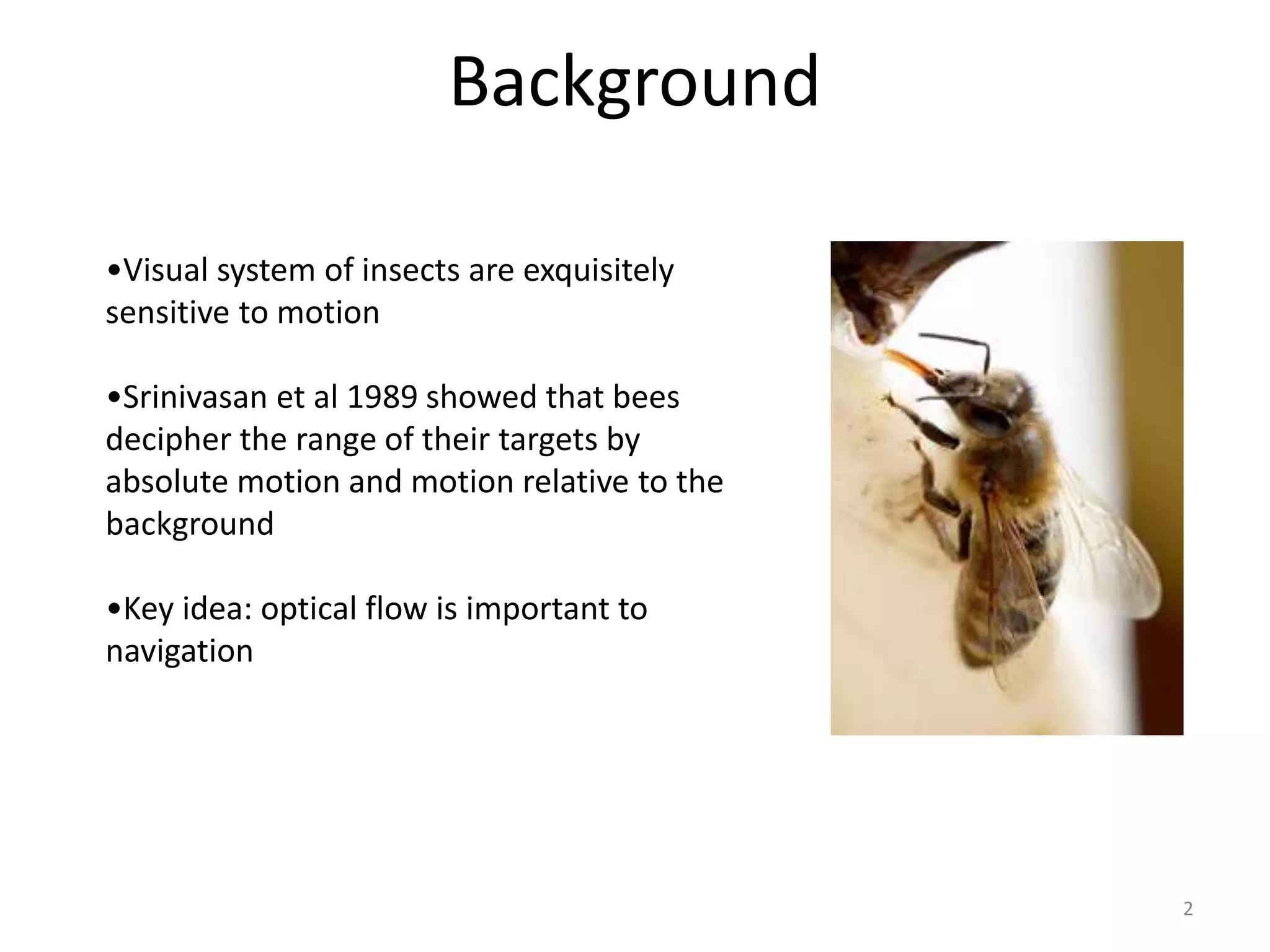
•Visual system of insects are exquisitely
sensitive to motion
•Srinivasan et al 1989 showed that bees
decipher the range of their targets by
absolute motion and motion relative to the
background
•Key idea: optical flow is important to
navigation
Motion Parallax in the Dorsal Stream
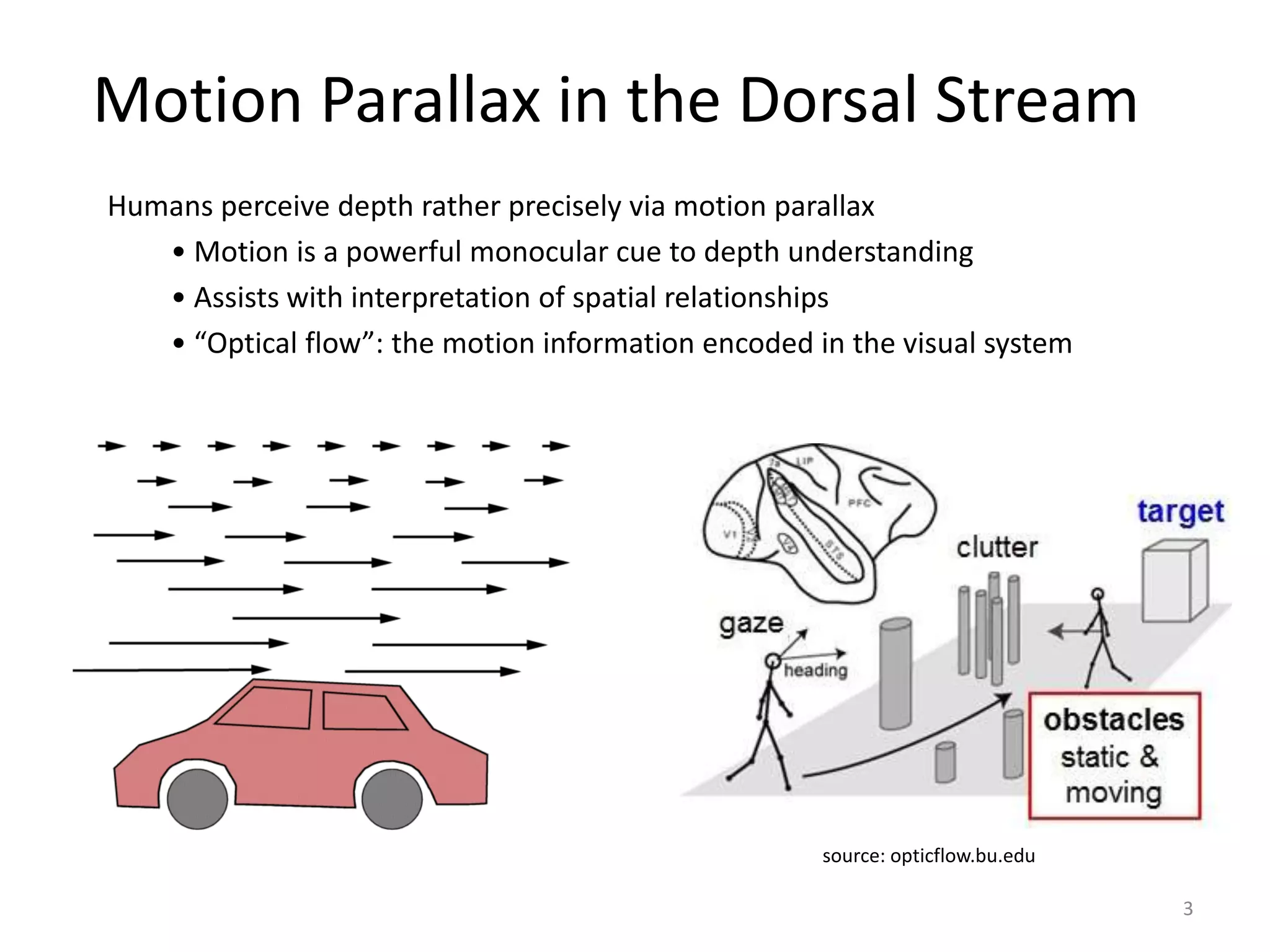
Humans perceive depth rather precisely via motion parallax
• Motion is a powerful monocular cue to depth understanding
• Assists with interpretation of spatial relationships
• “Optical flow”: the motion information encoded in the visual system
3
source: opticflow.bu.edu
Deep Learning
4
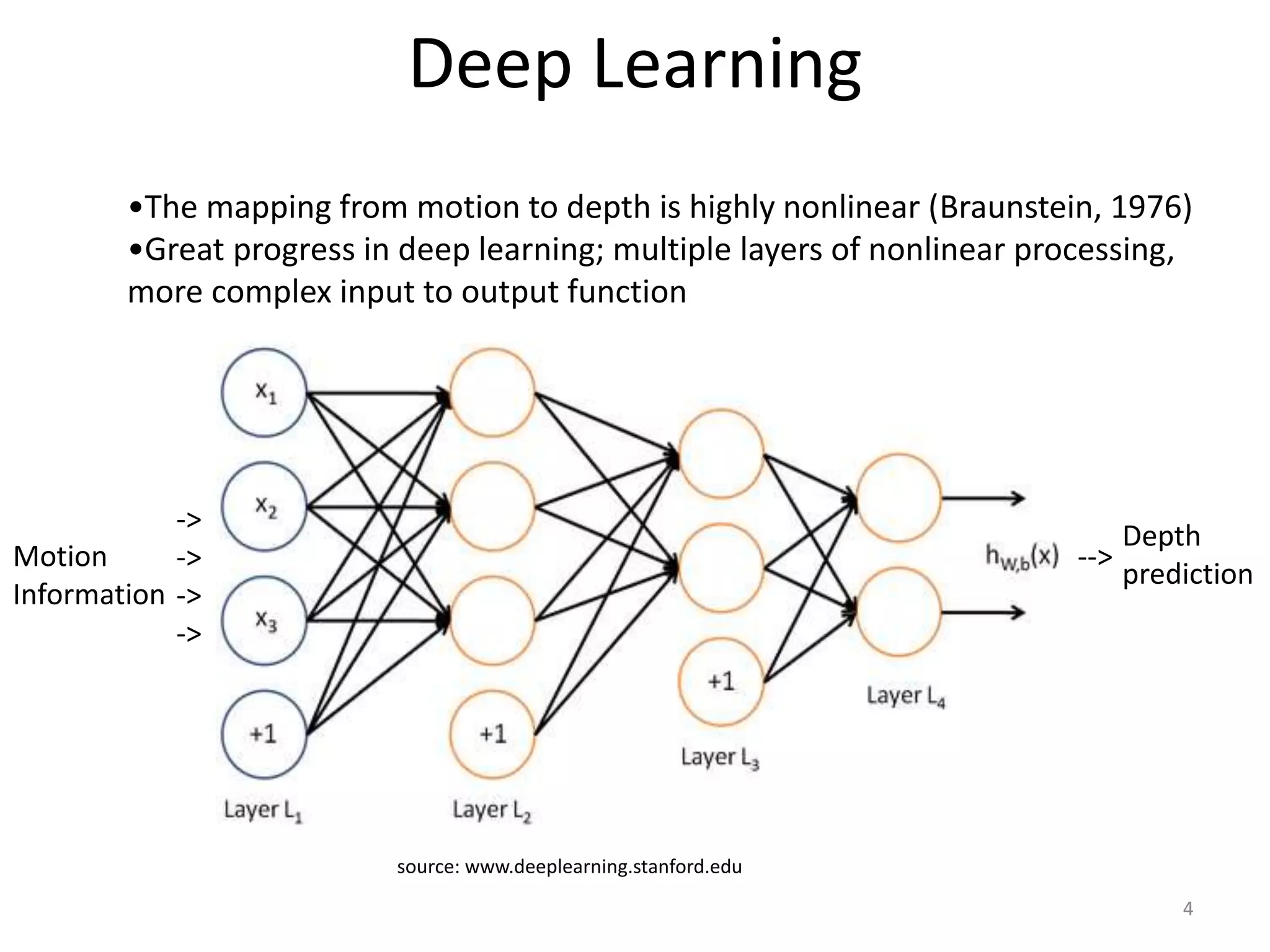
•The mapping from motion to depth is highly nonlinear (Braunstein, 1976)
•Great progress in deep learning; multiple layers of nonlinear processing,
more complex input to output function
source: www.deeplearning.stanford.edu
Motion
Information
Depth
prediction
->
->
->
->
-->
Computer Graphics
•Need labeled training data; videos do not have ground truth
depth
•Graphical scenes generated by a gaming engine provide large
number of training samples for supervised learning
5
A scene excerpt from our CryEngine forest database
RGB frame
ground truth depth map
6
MT Motion Model
• Hierarchical model of motion processing; alternate between template
matching and max pooling
• Convolutional learning of spatio-temporal features
• Extension of HMAX (Serre et al 2007)
Jhuang et al 2007
Population Responses
7
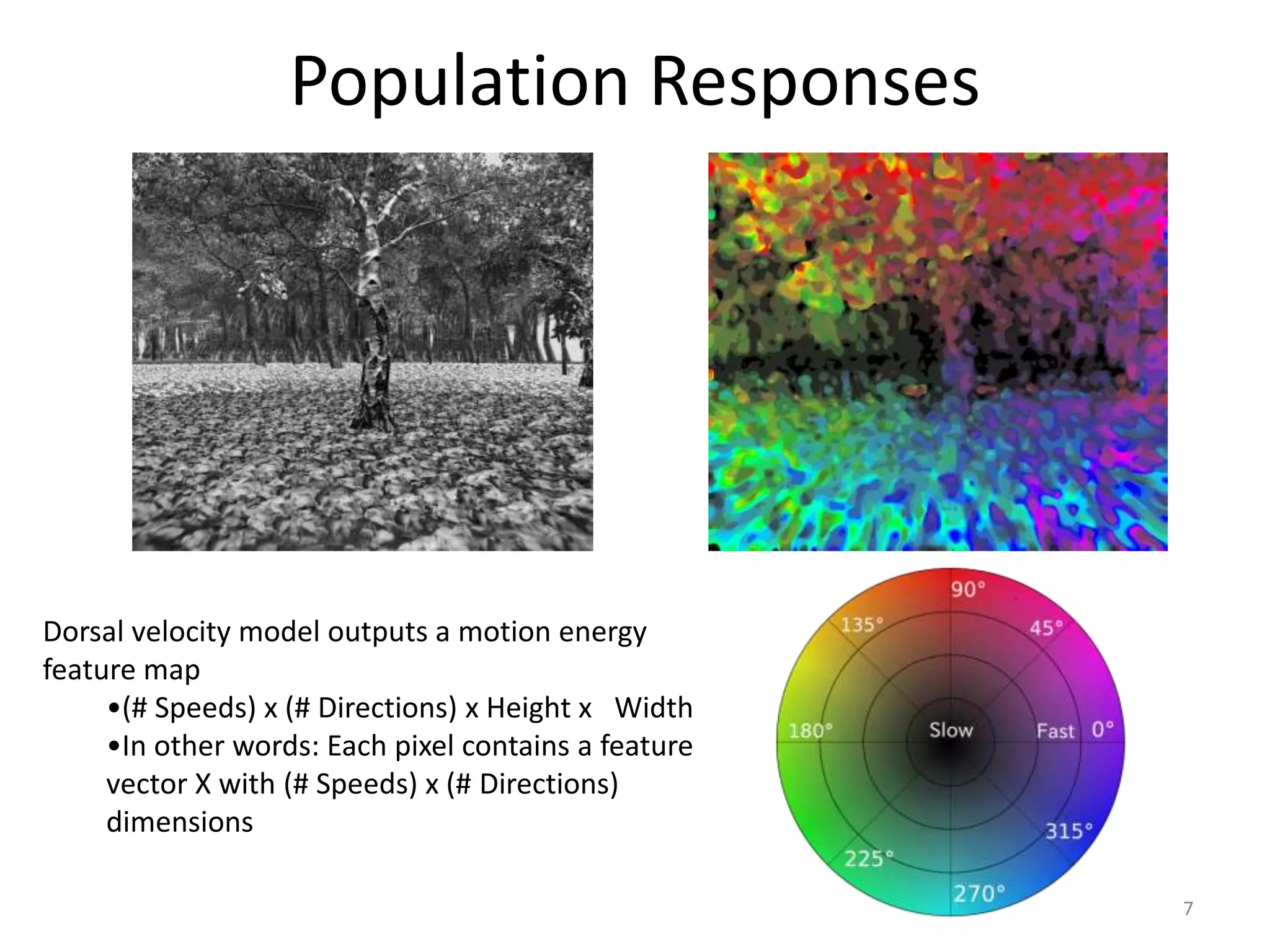
Dorsal velocity model outputs a motion energy
feature map
•(# Speeds) x (# Directions) x Height x Width
•In other words: Each pixel contains a feature
vector X with (# Speeds) x (# Directions)
dimensions
8
Deep Belief Networks
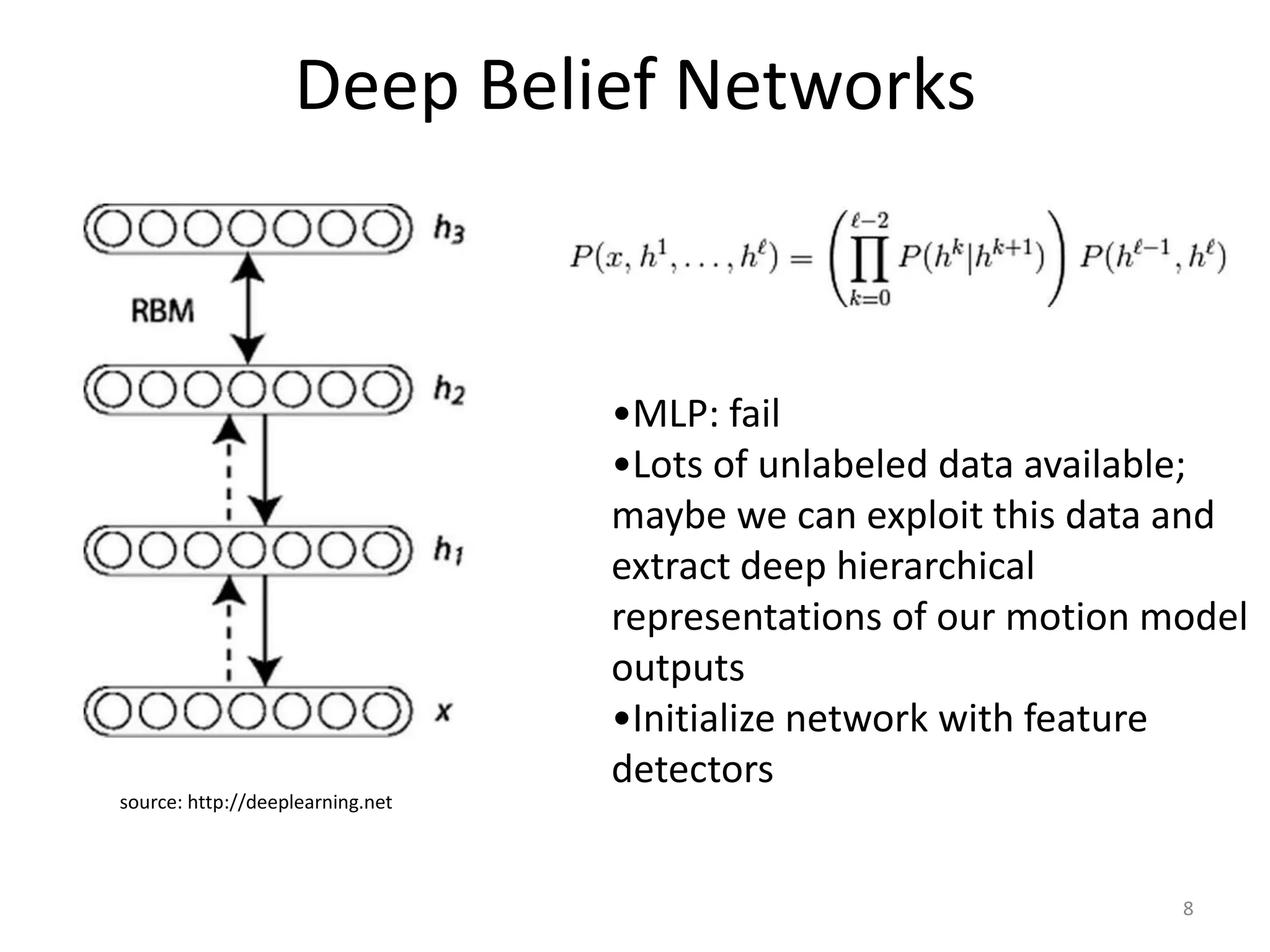
•MLP: fail
•Lots of unlabeled data available;
maybe we can exploit this data and
extract deep hierarchical
representations of our motion model
outputs
•Initialize network with feature
detectors
source: http://deeplearning.net
The RBM Model
9
Maximum likelihood learning: update model parameters to maximize the
likelihood of our training data
Standard RBM:
Gaussian-Bernoulli RBM:
P(v,h) = (1/Z)*exp(-E(v,h))
We then create a new “free energy” version
which sums over all possible hidden states
P(v) = (1/Z)*exp(-F(v))
source: http://deeplearning.net
Justifying Greedy Layer-Wise Pre-Training
10
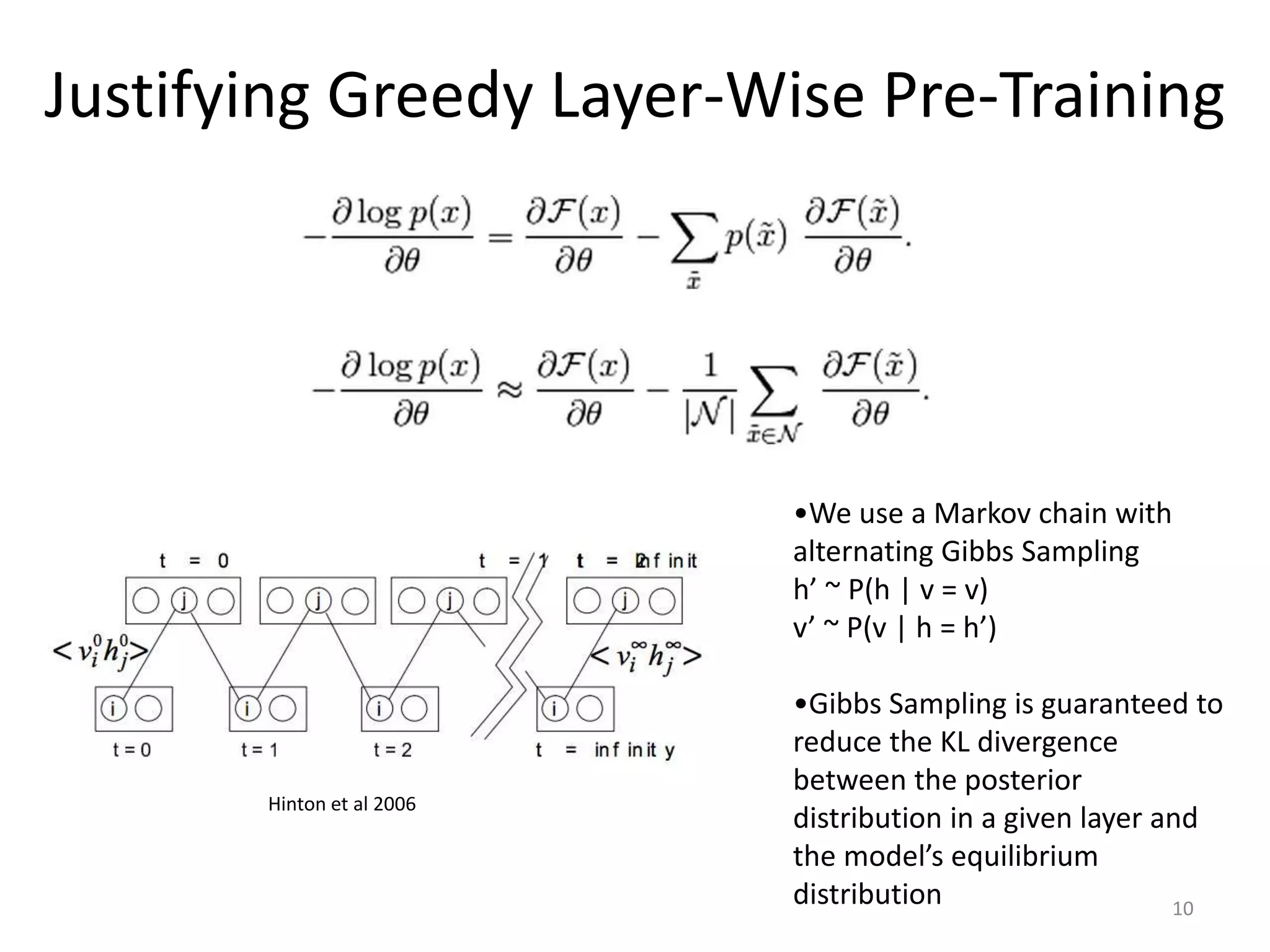
•We use a Markov chain with
alternating Gibbs Sampling
h’ ~ P(h | v = v)
v’ ~ P(v | h = h’)
•Gibbs Sampling is guaranteed to
reduce the KL divergence
between the posterior
distribution in a given layer and
the model’s equilibrium
distribution
Hinton et al 2006
The DBN
11
• The data: feature vectors have 72 elements, tuned to 9
different speeds and 8 directions (9*8 = 72)
• DBN takes in 3x3 pixel window
• 3 Hidden layers of 800 units; sigmoidal activation
• Linear output layer
Technicalities:
•Mini-batch training with batch size of 5000
•Sparse initialization scheme
•RMSprop learning rule (regularized mean squares)
•Backpropagation fine-tuning with dropout, dropping 20% of units at each
layer except for the input layer
•Geometrically decaying learning rate (LR = 0.998*LR at each epoch)
Results
12
DBN Linear RegressionGround Truth
test set R2: 0.445 test set R2: 0.240
13
MLP (sparse
initialization)
single-pixel
linear
regression
3x3 window
linear
regression
single-pixel DBN
3x3 window
DBN
0
0.05
0.1
0.15
0.2
0.25
0.3
0.35
0.4
0.45
0.5
0 1 2 3 4 5 6
R^2Score R^2 Score per Model
Markov Random Field Smoothing
Receptive field can be a powerful tool for decoding
14
MRF defined by two potential functions:
1) Φ = ∑_i [ (w • x_i − d_i) ^ 2 ]
2) Ψ = ∑_<i,j> [ (d_i − d_j)^2 /( (d_i − d_j)^2 + 1) ) ]
(note: <i,j> = all neighboring pairs i,j)
P(d | x ; alpha, w) = (1/Z) * exp(− (alpha*Ψ + Φ)).
Peter Orchard, University of Edinburgh
ground truth original prediction: 0.595 MRF prediction: 0.630
Drone Test
15
16
Future Work
• Increase pre-training dataset
• Real video labeled data with XBOX Kinect
• Down-sample motion features and ground
truth
17
Thanks!
• Thomas Serre
• Stuart Geman
• David Mely
• Youssef Barhomi
18
Questions?
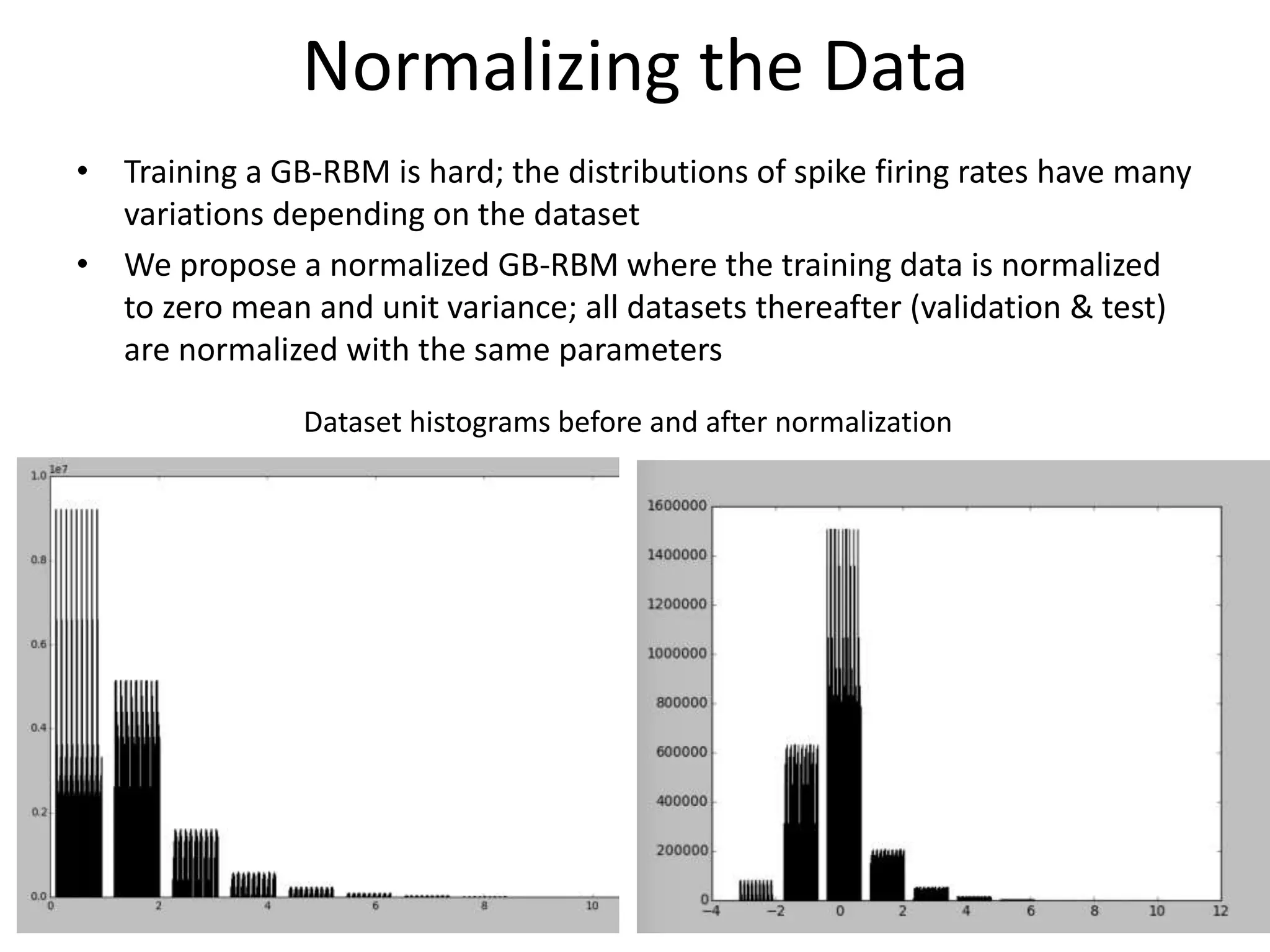
Normalizing the Data
• Training a GB-RBM is hard; the distributions of spike firing rates have many
variations depending on the dataset
• We propose a normalized GB-RBM where the training data is normalized
to zero mean and unit variance; all datasets thereafter (validation & test)
are normalized with the same parameters
19
Dataset histograms before and after normalization

Thesis Presentation

  • 1.
    A Deep BeliefNetwork Approach to Learning Depth from Optical Flow Reuben Feinman 1 Applied Mathematics Honors Thesis by
  • 2.
    Background 2 •Visual system ofinsects are exquisitely sensitive to motion •Srinivasan et al 1989 showed that bees decipher the range of their targets by absolute motion and motion relative to the background •Key idea: optical flow is important to navigation
  • 3.
    Motion Parallax inthe Dorsal Stream Humans perceive depth rather precisely via motion parallax • Motion is a powerful monocular cue to depth understanding • Assists with interpretation of spatial relationships • “Optical flow”: the motion information encoded in the visual system 3 source: opticflow.bu.edu
  • 4.
    Deep Learning 4 •The mappingfrom motion to depth is highly nonlinear (Braunstein, 1976) •Great progress in deep learning; multiple layers of nonlinear processing, more complex input to output function source: www.deeplearning.stanford.edu Motion Information Depth prediction -> -> -> -> -->
  • 5.
    Computer Graphics •Need labeledtraining data; videos do not have ground truth depth •Graphical scenes generated by a gaming engine provide large number of training samples for supervised learning 5 A scene excerpt from our CryEngine forest database RGB frame ground truth depth map
  • 6.
    6 MT Motion Model •Hierarchical model of motion processing; alternate between template matching and max pooling • Convolutional learning of spatio-temporal features • Extension of HMAX (Serre et al 2007) Jhuang et al 2007
  • 7.
    Population Responses 7 Dorsal velocitymodel outputs a motion energy feature map •(# Speeds) x (# Directions) x Height x Width •In other words: Each pixel contains a feature vector X with (# Speeds) x (# Directions) dimensions
  • 8.
    8 Deep Belief Networks •MLP:fail •Lots of unlabeled data available; maybe we can exploit this data and extract deep hierarchical representations of our motion model outputs •Initialize network with feature detectors source: http://deeplearning.net
  • 9.
    The RBM Model 9 Maximumlikelihood learning: update model parameters to maximize the likelihood of our training data Standard RBM: Gaussian-Bernoulli RBM: P(v,h) = (1/Z)*exp(-E(v,h)) We then create a new “free energy” version which sums over all possible hidden states P(v) = (1/Z)*exp(-F(v)) source: http://deeplearning.net
  • 10.
    Justifying Greedy Layer-WisePre-Training 10 •We use a Markov chain with alternating Gibbs Sampling h’ ~ P(h | v = v) v’ ~ P(v | h = h’) •Gibbs Sampling is guaranteed to reduce the KL divergence between the posterior distribution in a given layer and the model’s equilibrium distribution Hinton et al 2006
  • 11.
    The DBN 11 • Thedata: feature vectors have 72 elements, tuned to 9 different speeds and 8 directions (9*8 = 72) • DBN takes in 3x3 pixel window • 3 Hidden layers of 800 units; sigmoidal activation • Linear output layer Technicalities: •Mini-batch training with batch size of 5000 •Sparse initialization scheme •RMSprop learning rule (regularized mean squares) •Backpropagation fine-tuning with dropout, dropping 20% of units at each layer except for the input layer •Geometrically decaying learning rate (LR = 0.998*LR at each epoch)
  • 12.
    Results 12 DBN Linear RegressionGroundTruth test set R2: 0.445 test set R2: 0.240
  • 13.
    13 MLP (sparse initialization) single-pixel linear regression 3x3 window linear regression single-pixelDBN 3x3 window DBN 0 0.05 0.1 0.15 0.2 0.25 0.3 0.35 0.4 0.45 0.5 0 1 2 3 4 5 6 R^2Score R^2 Score per Model
  • 14.
    Markov Random FieldSmoothing Receptive field can be a powerful tool for decoding 14 MRF defined by two potential functions: 1) Φ = ∑_i [ (w • x_i − d_i) ^ 2 ] 2) Ψ = ∑_<i,j> [ (d_i − d_j)^2 /( (d_i − d_j)^2 + 1) ) ] (note: <i,j> = all neighboring pairs i,j) P(d | x ; alpha, w) = (1/Z) * exp(− (alpha*Ψ + Φ)). Peter Orchard, University of Edinburgh ground truth original prediction: 0.595 MRF prediction: 0.630
  • 15.
  • 16.
  • 17.
    Future Work • Increasepre-training dataset • Real video labeled data with XBOX Kinect • Down-sample motion features and ground truth 17
  • 18.
    Thanks! • Thomas Serre •Stuart Geman • David Mely • Youssef Barhomi 18 Questions?
  • 19.
    Normalizing the Data •Training a GB-RBM is hard; the distributions of spike firing rates have many variations depending on the dataset • We propose a normalized GB-RBM where the training data is normalized to zero mean and unit variance; all datasets thereafter (validation & test) are normalized with the same parameters 19 Dataset histograms before and after normalization