Download as PDF, PPTX
![Lecture 9—Non-linear systems
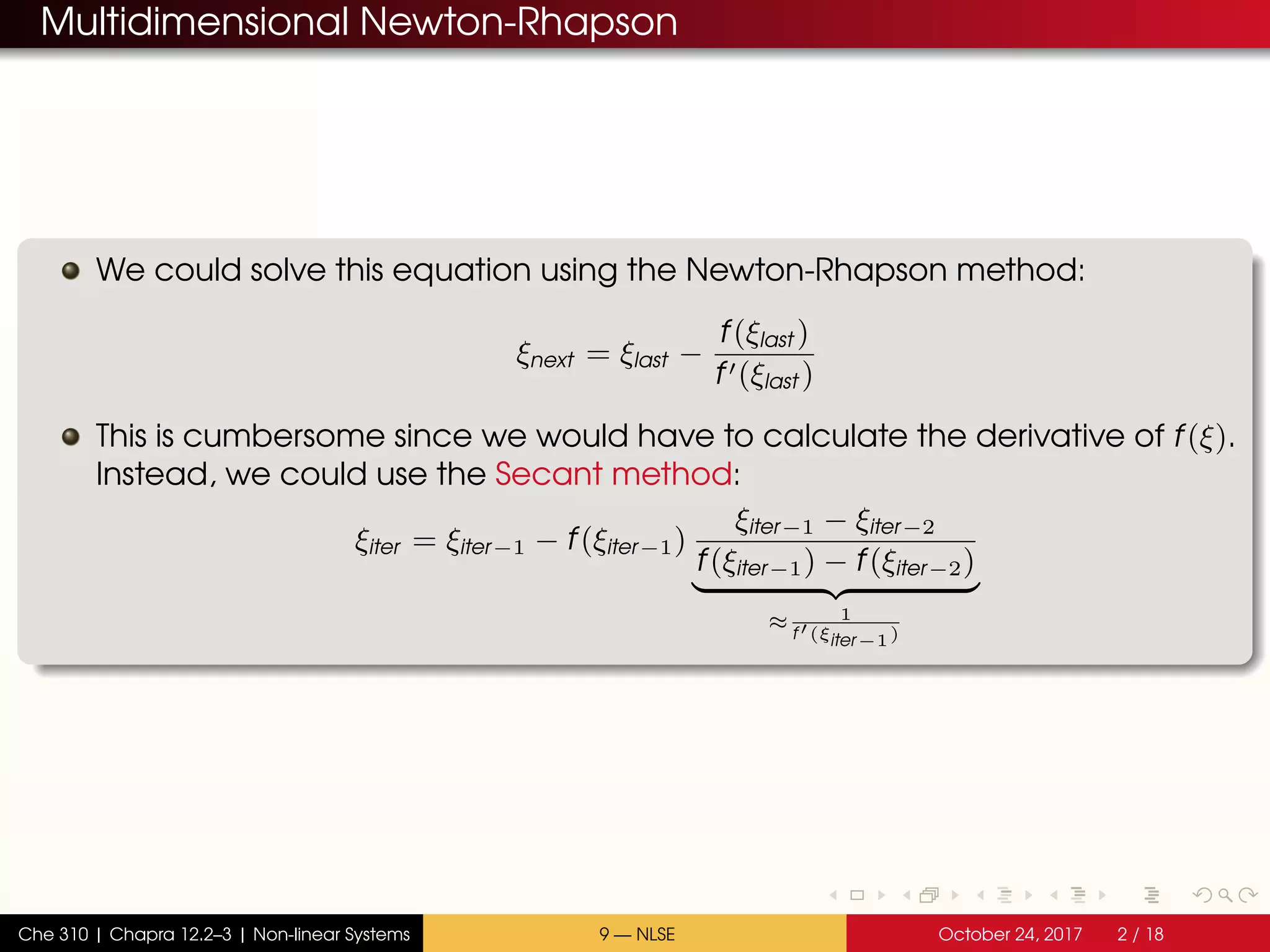
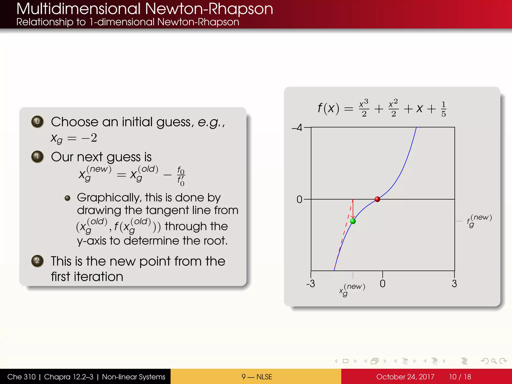
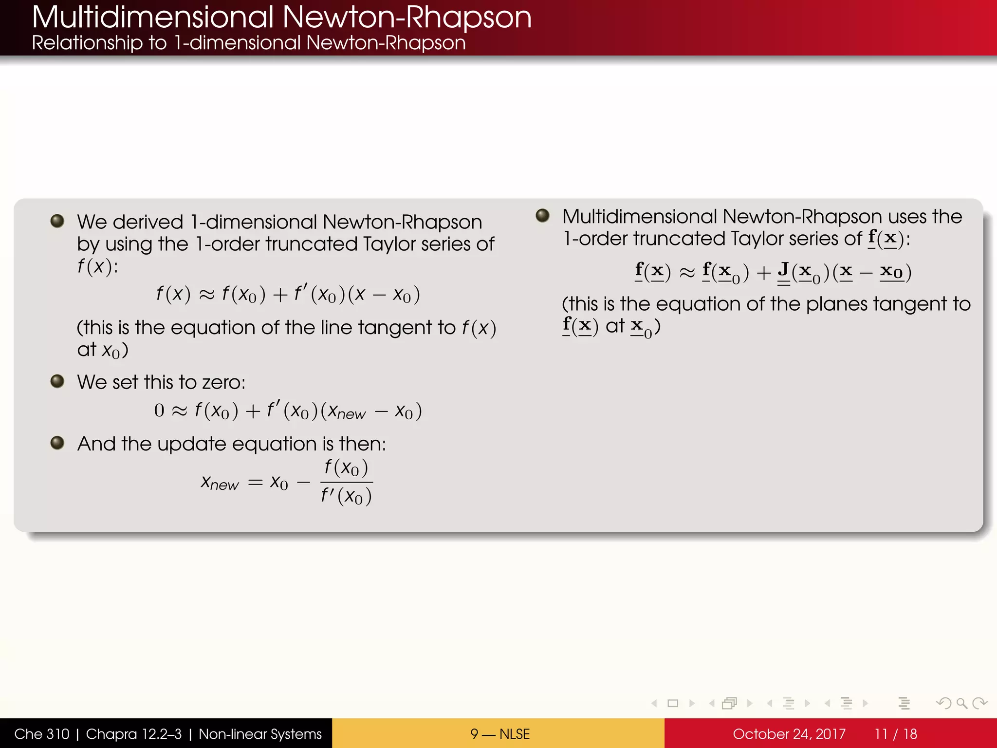
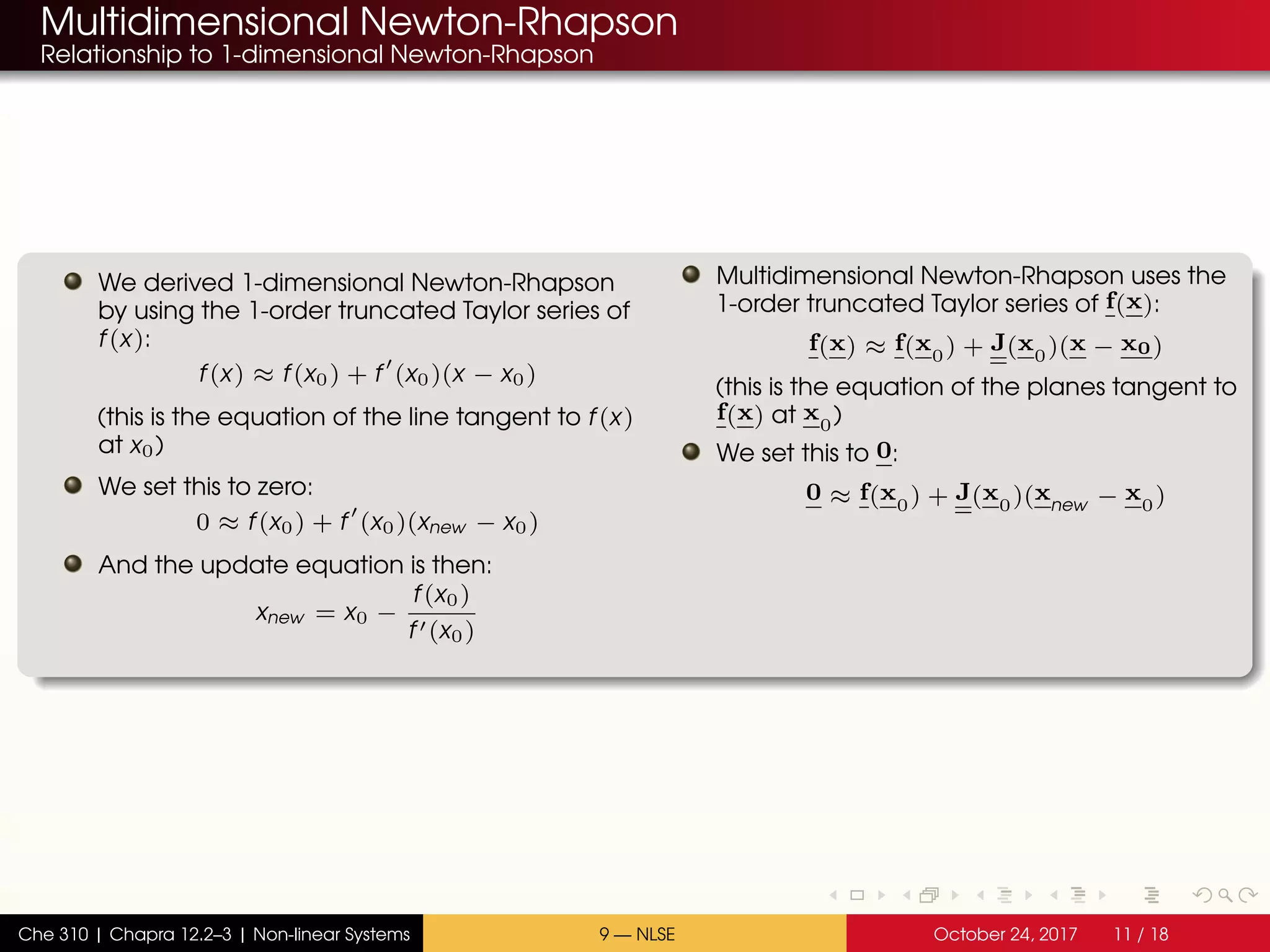
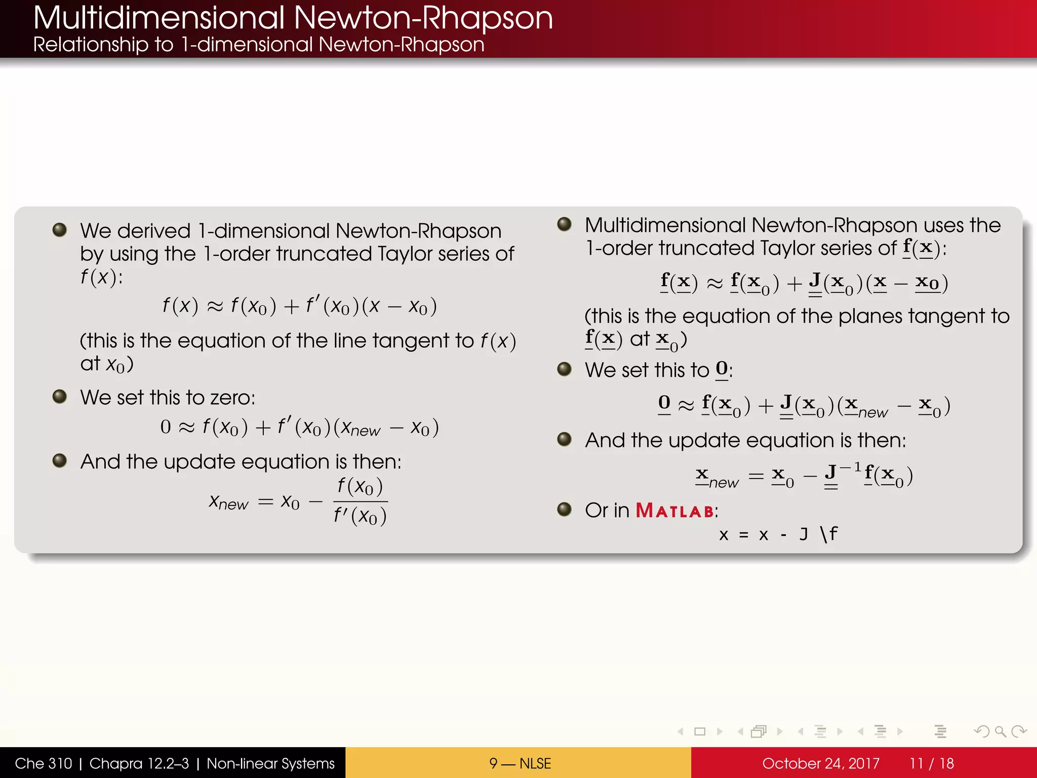
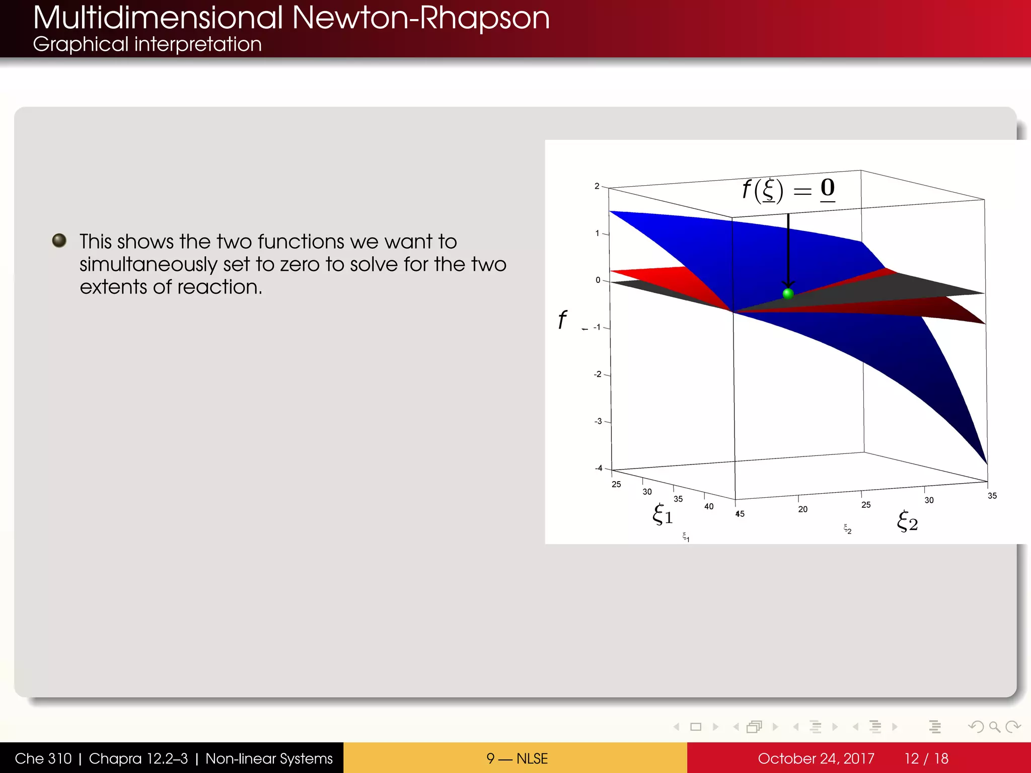
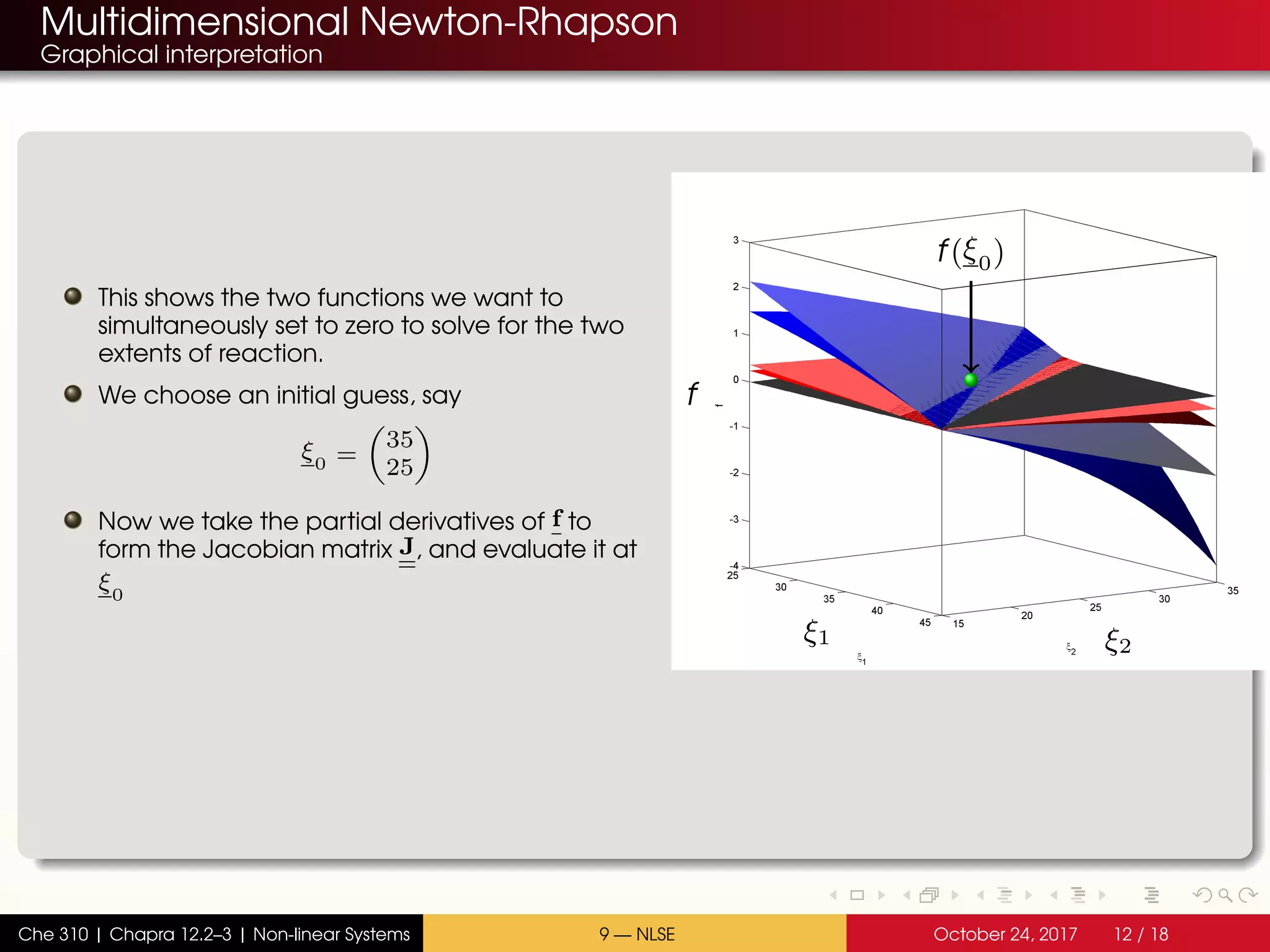
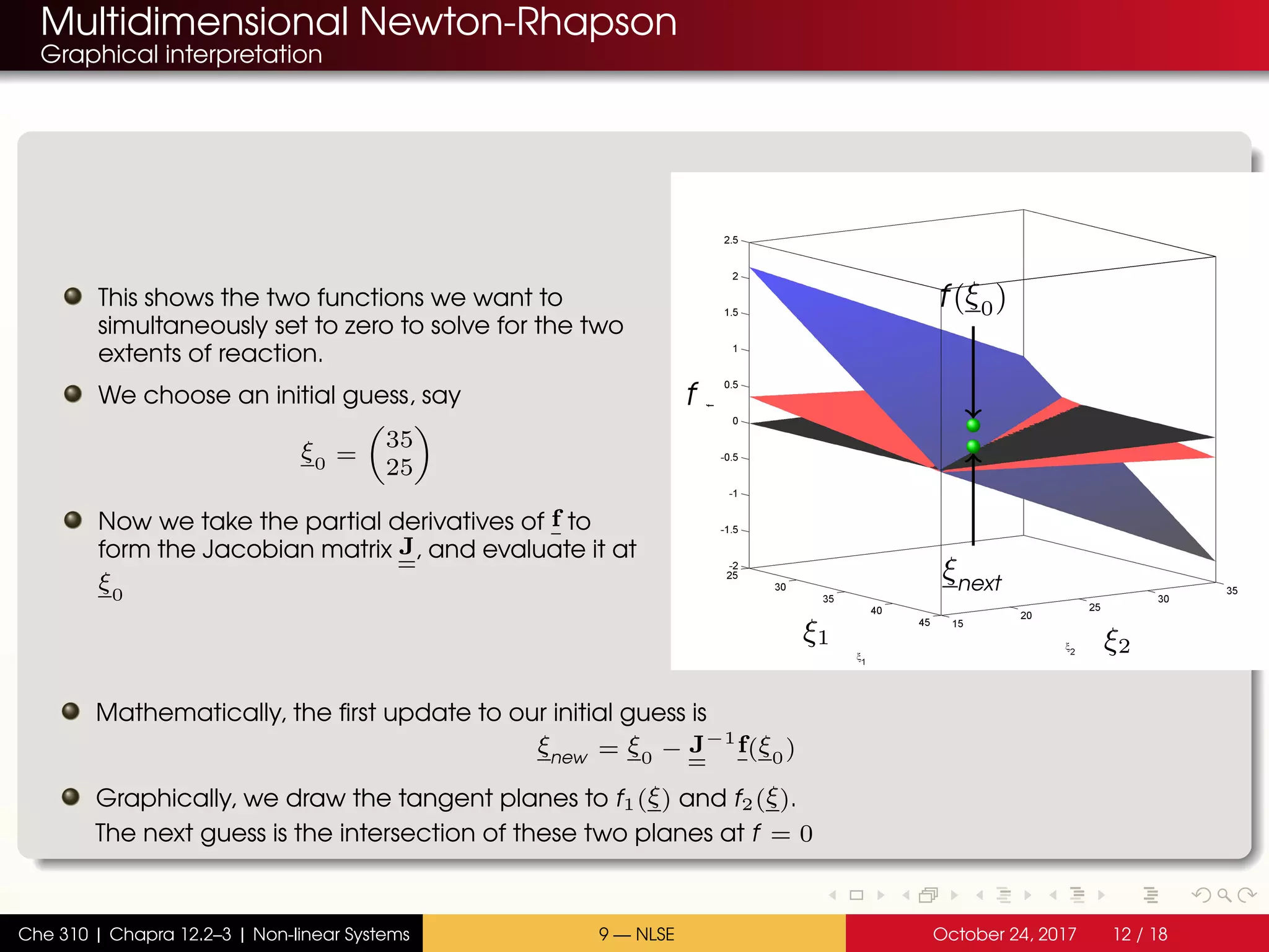
Multidimensional Newton-Rhapson
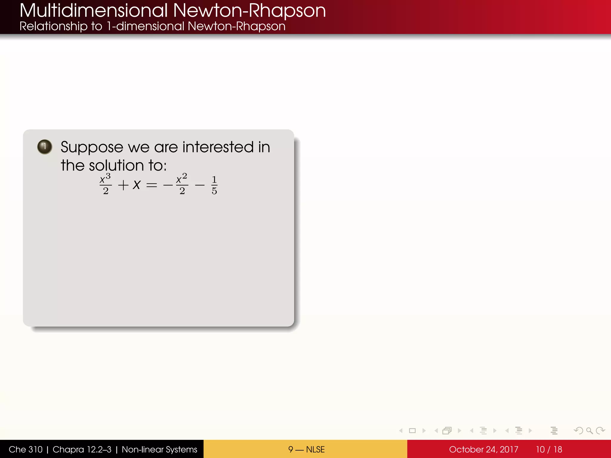
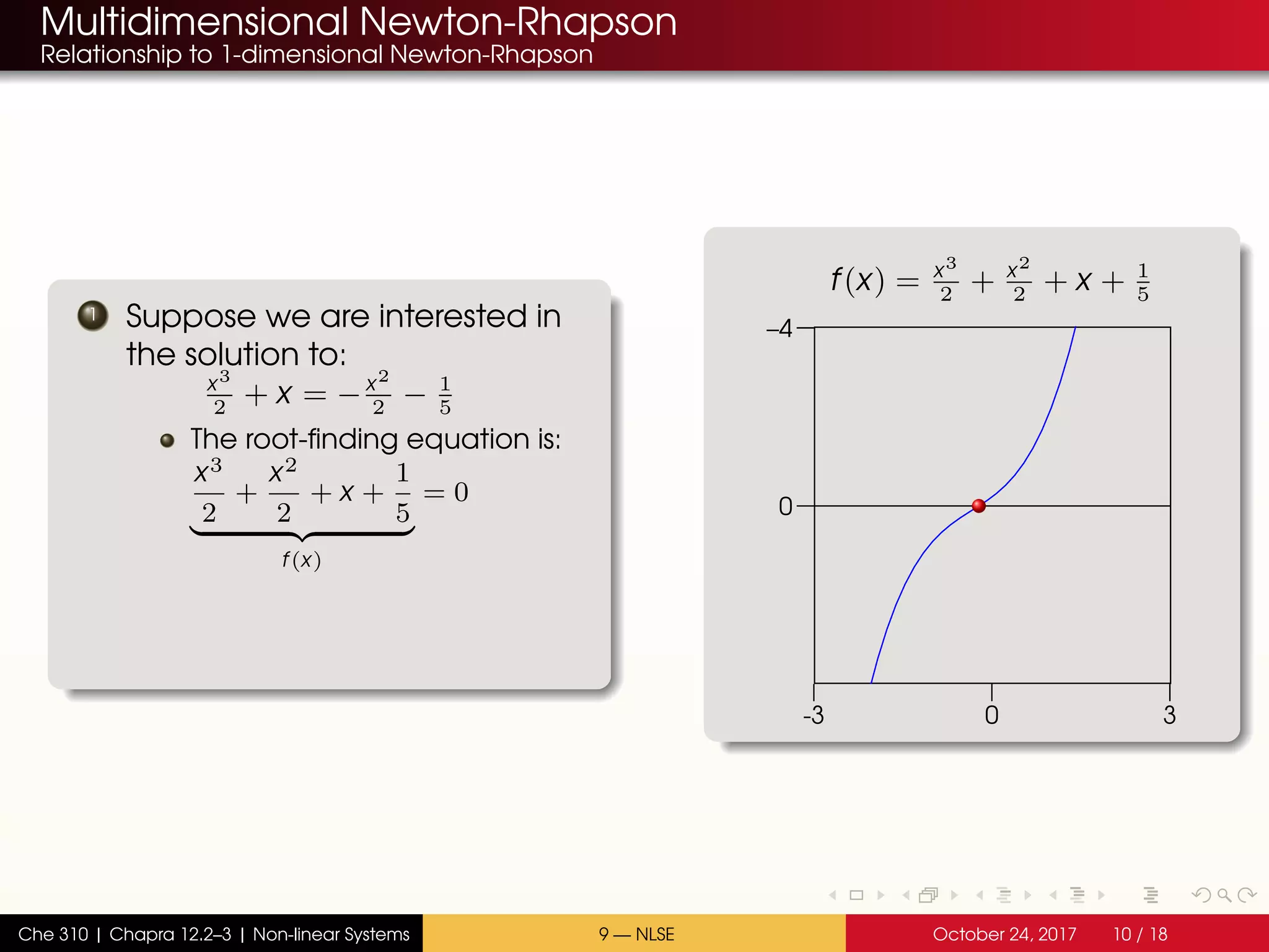
We have dealt with the solution of a single non-linear equation and the
simultaneous solution of multiple linear equations. Now we are going to look
at the simultaneous solution of solving multiple non-linear equations.
To start, let’s consider a single equilibrium reaction:
A −−→←−− B + 2 C
The stoichiometric coefficients are s = [−1 12] for A, B, and C.
To find the equilibrium conversion, solve for the reaction coordinate using
the single equilibrium relationship:
f(ξ) = K −
nB,in+ξ
ntot
in
+2ξ
nC,in+2ξ
ntot
in
+2ξ
2
nA,in−ξ
ntot
in
+2ξ
The value of ξ that satisfies f(ξ) = 0 is the extent of reaction that satisfies the
equilibrium relationship.
Che 310 | Chapra 12.2–3 | Non-linear Systems 9 — NLSE October 24, 2017 1 / 18](https://image.slidesharecdn.com/lecture9f17-171024134123/75/Lecture-9-f17-1-2048.jpg)
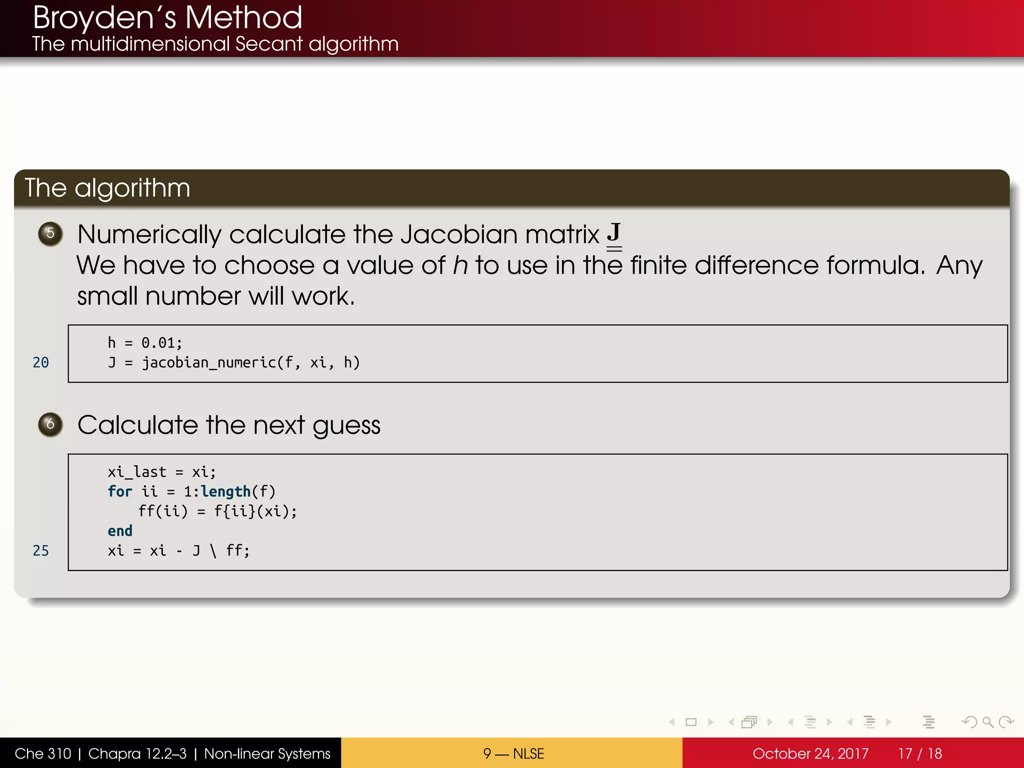
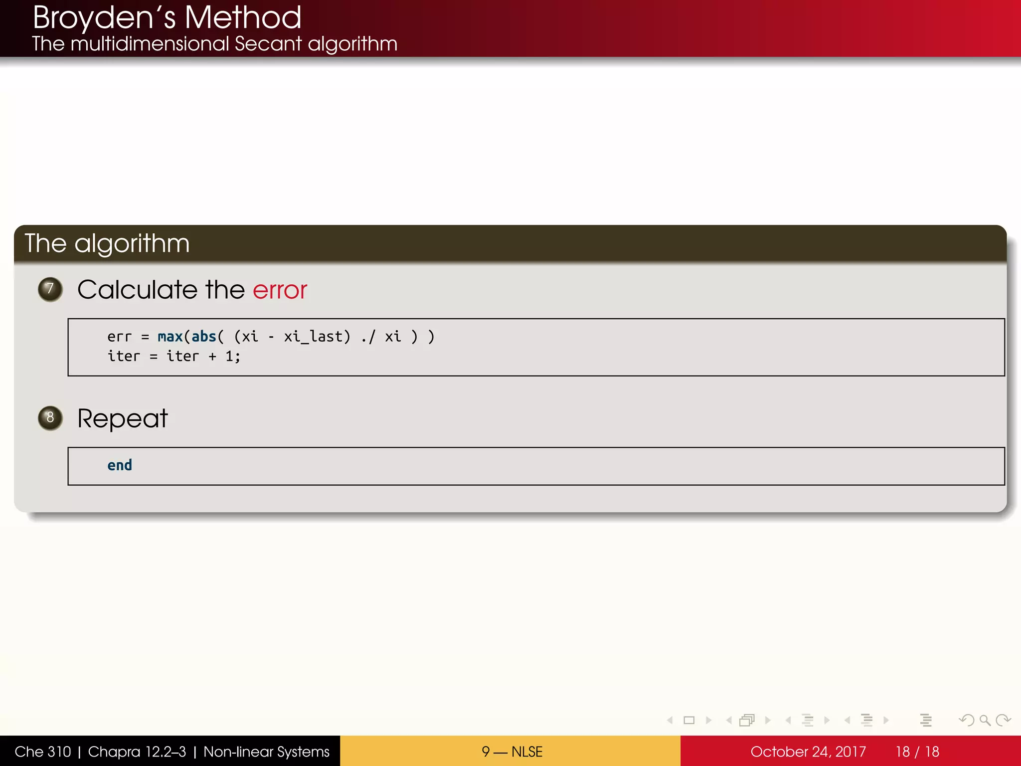
![Broyden’s Method
The multidimensional Secant algorithm
The algorithm
1 Enter all of the non-linear functions as a single
function handle:
S1 = [ 2 1 -1 0 ];
S2 = [ 1 0 -1 1 ];
K = [ 0.32 2.6 ];
n_tot = @(xi) sum(n_in) + ...
5 sum(S1) .* xi(1) + ...
sum(S2) .* xi(2)
n_out = @(xi) n_in + ...
S1 .* xi(1) + ...
S2 .* xi(2)
10 f = @(xi) ...
[ K(1) - ...
prod( n_out(xi).^S1 ) ...
/ n_tot(xi).^sum(S1) ; ...
K(2) - ...
15 prod( n_out(xi).^S2 ) ...
/ n_tot(xi).^sum(S2) ]
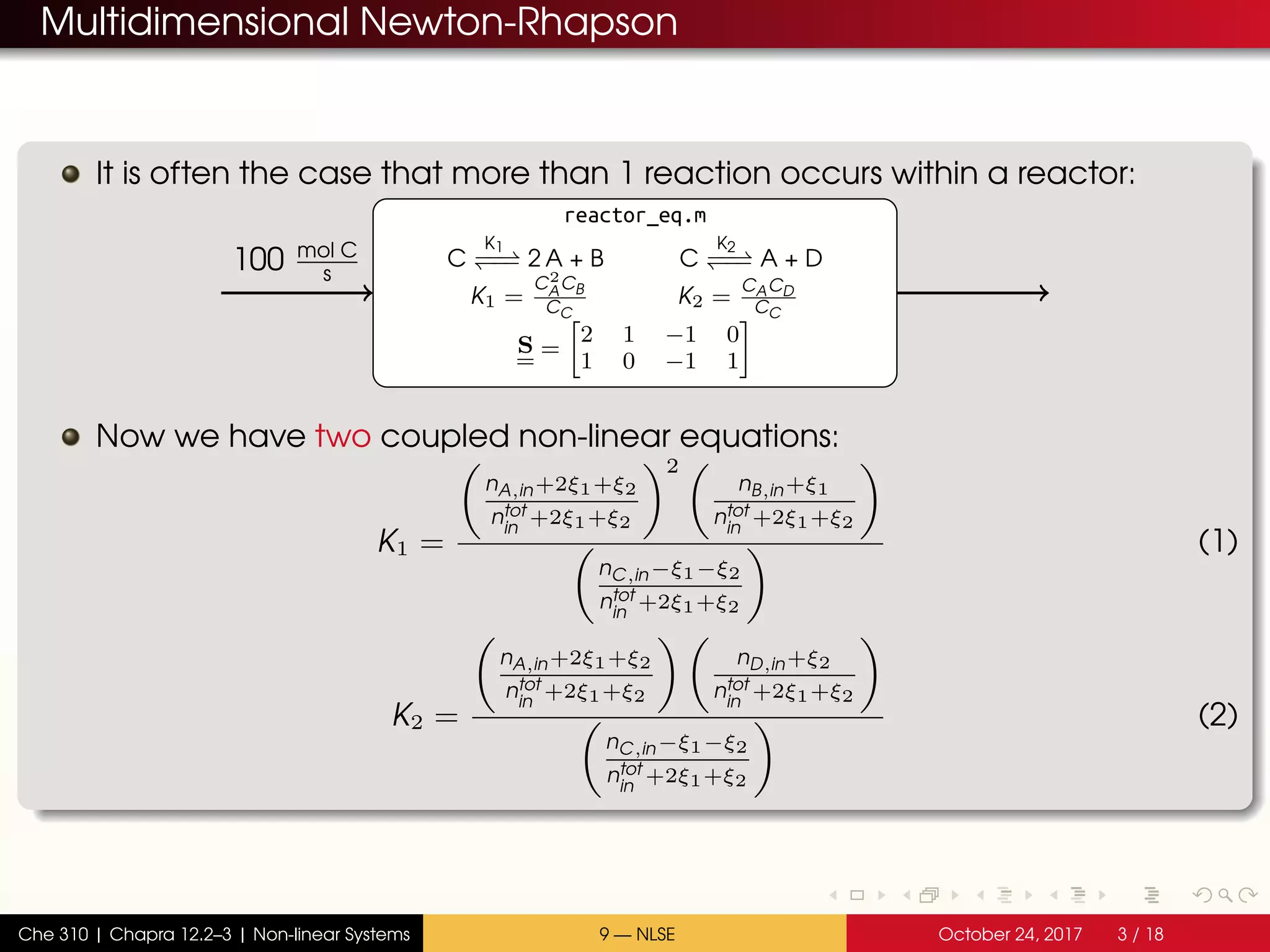
The reactions:
C
K1 = 0.32
−−−−−−−−−−−−−−−− 2 A + B
C
K2 = 2.60
−−−−−−−−−−−−−−−− A + D
S1 = [2 1 −1 0]
S2 = [1 0 −1 1]
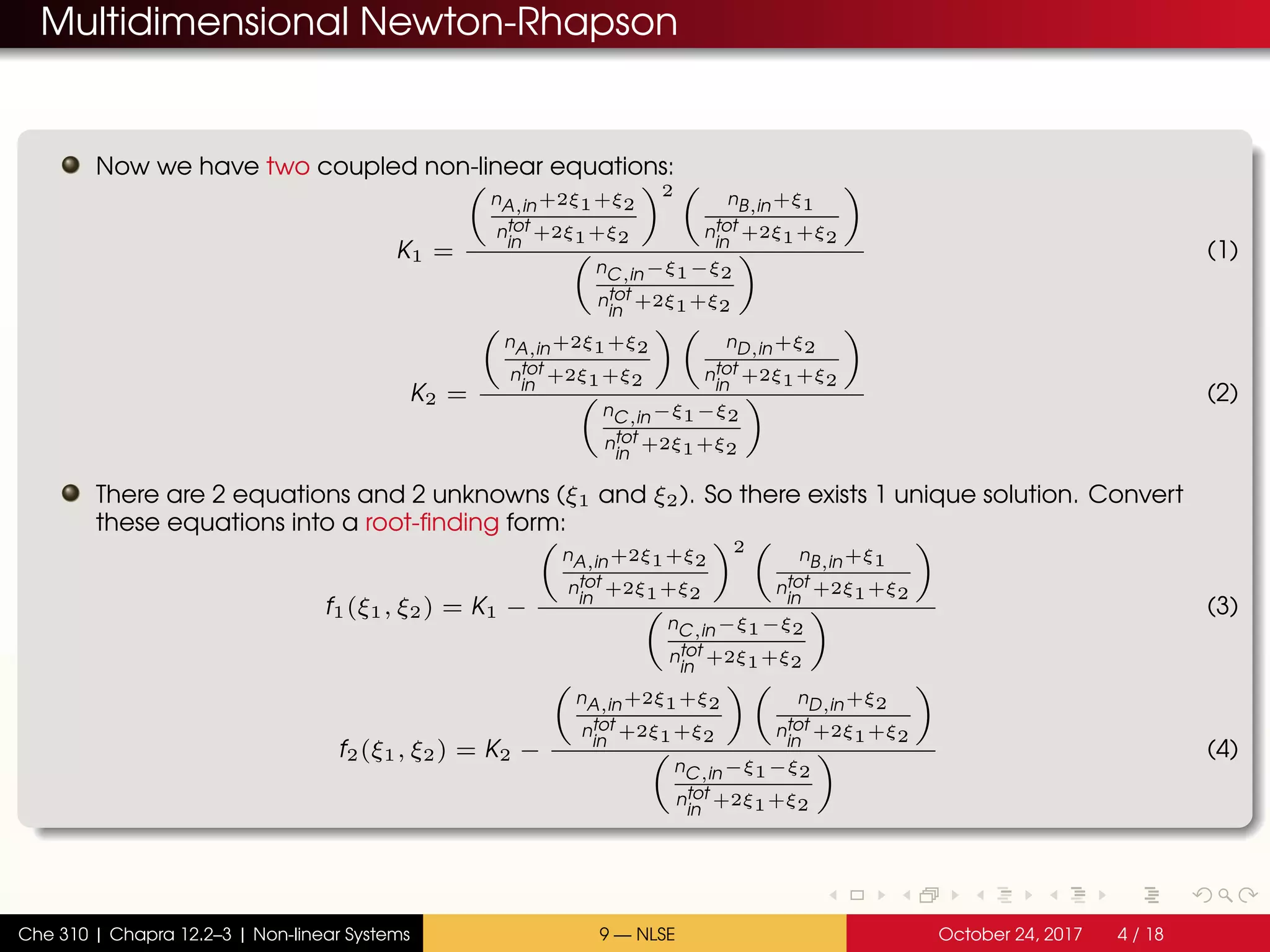
The non-linear equations:
K1 =
C2
A
CB
CC
K2 =
CACD
CC
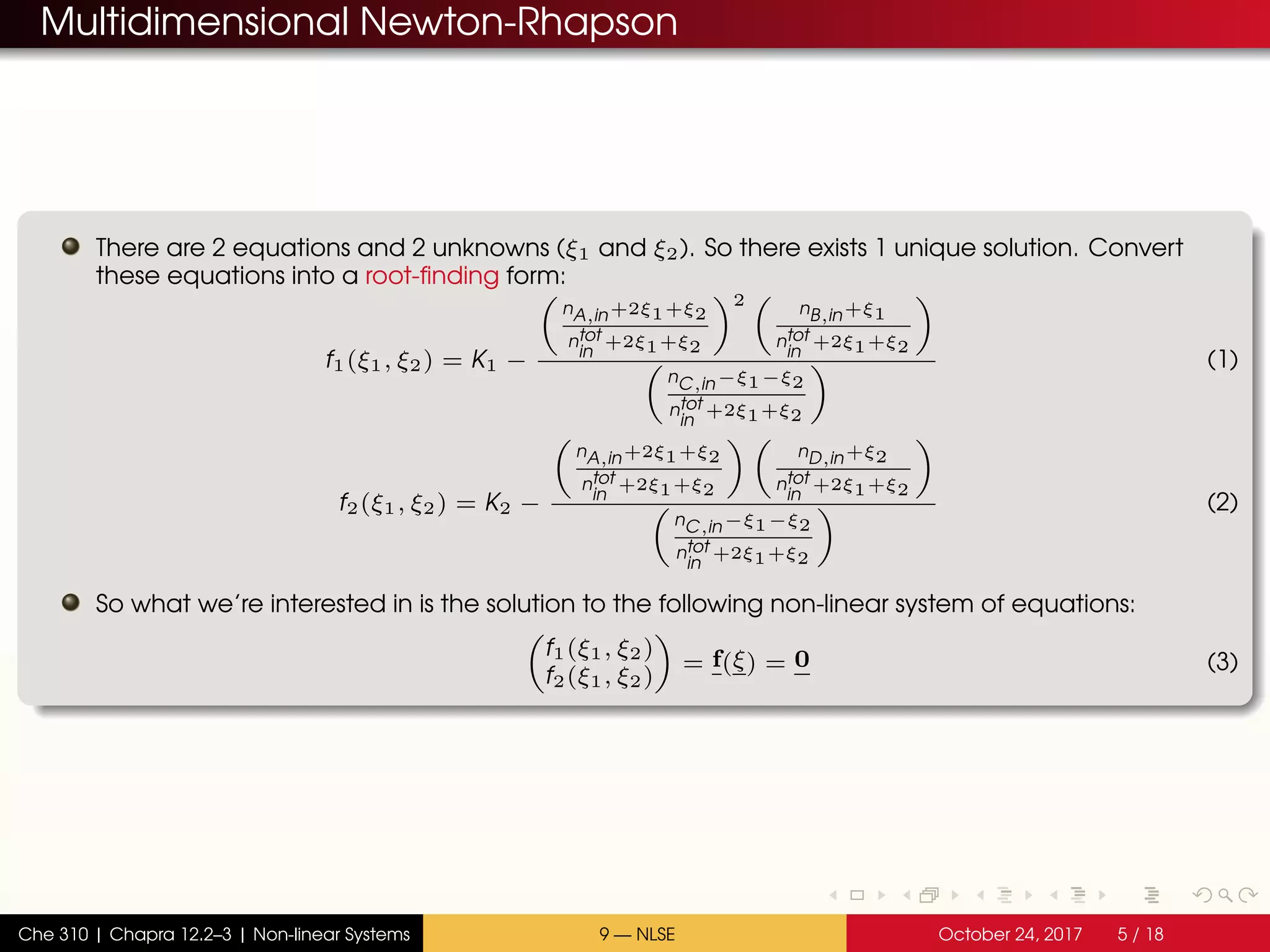
The root-finding functions:
f1(ξ1, ξ2) = K1 −
nA,in+2ξ1+ξ2
ntot
in
+2ξ1+ξ2
2
nB,in+ξ1
ntot
in
+2ξ1+ξ2
nC,in−ξ1−ξ2
ntot
in
+2ξ1+ξ2
f2(ξ1, ξ2) = K2 −
nA,in+2ξ1+ξ2
ntot
in
+2ξ1+ξ2
nD,in+ξ2
ntot
in
+2ξ1+ξ2
nC,in−ξ1−ξ2
ntot
in
+2ξ1+ξ2
Che 310 | Chapra 12.2–3 | Non-linear Systems 9 — NLSE October 24, 2017 14 / 18](https://image.slidesharecdn.com/lecture9f17-171024134123/75/Lecture-9-f17-31-2048.jpg)
![Broyden’s Method
The multidimensional Secant algorithm
The algorithm
2 Choose an initial guess
xi0 = [ 35; 25] ;
It is always helpful to have some idea of the neighborhood of the solution.
In this example, we know that component C is reacting. At least 0 moles of C will be
converted.
Therefore, our initial guesses should be positive.
Also, no more than nC,in moles of C can be converted. There are two reactions, so the
total number of moles of C consumed will be ξ1 + ξ2.
If 100 moles of C are entering the reactor, then ξ1 + ξ2 < 100
Che 310 | Chapra 12.2–3 | Non-linear Systems 9 — NLSE October 24, 2017 15 / 18](https://image.slidesharecdn.com/lecture9f17-171024134123/75/Lecture-9-f17-32-2048.jpg)

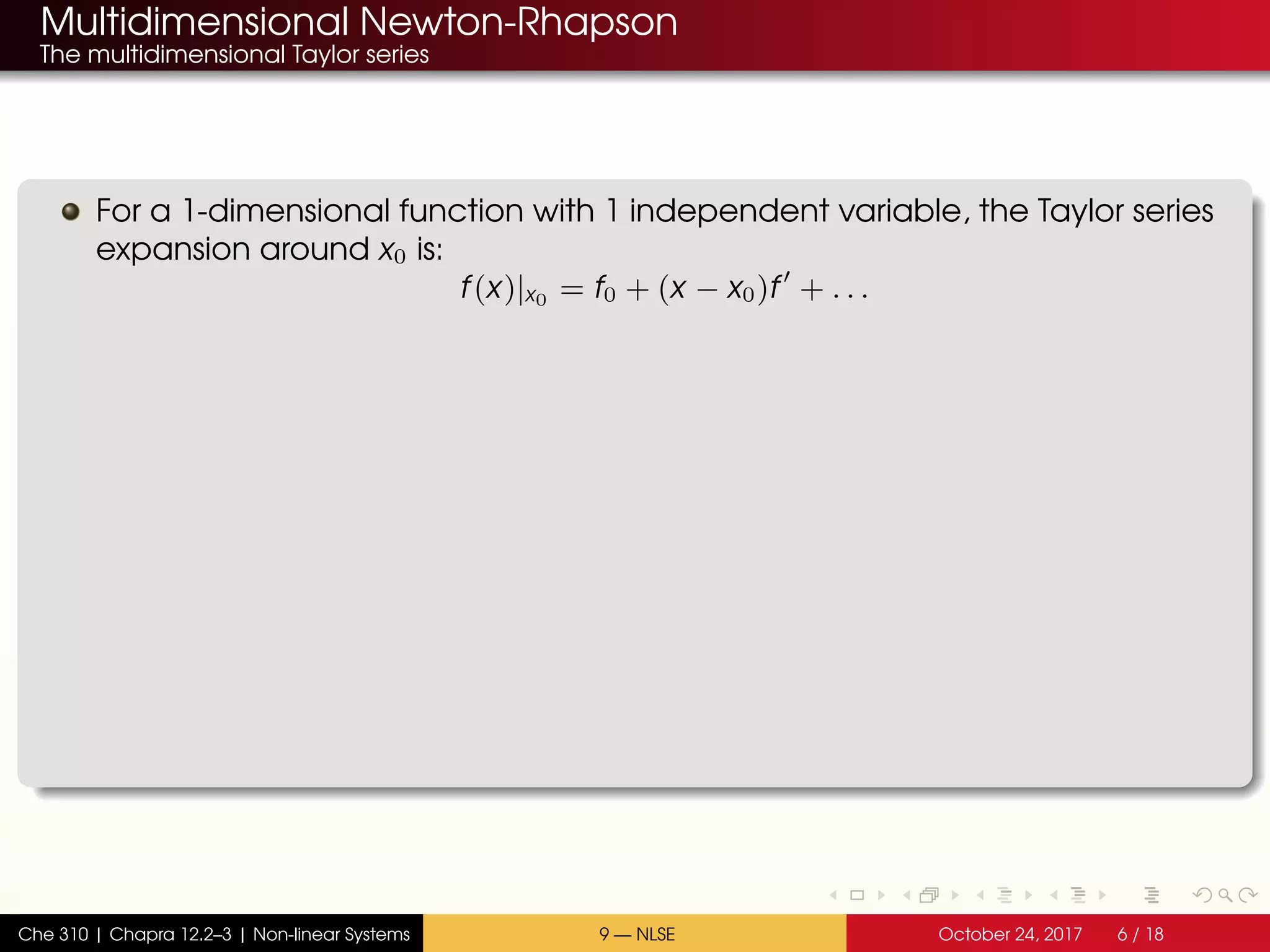
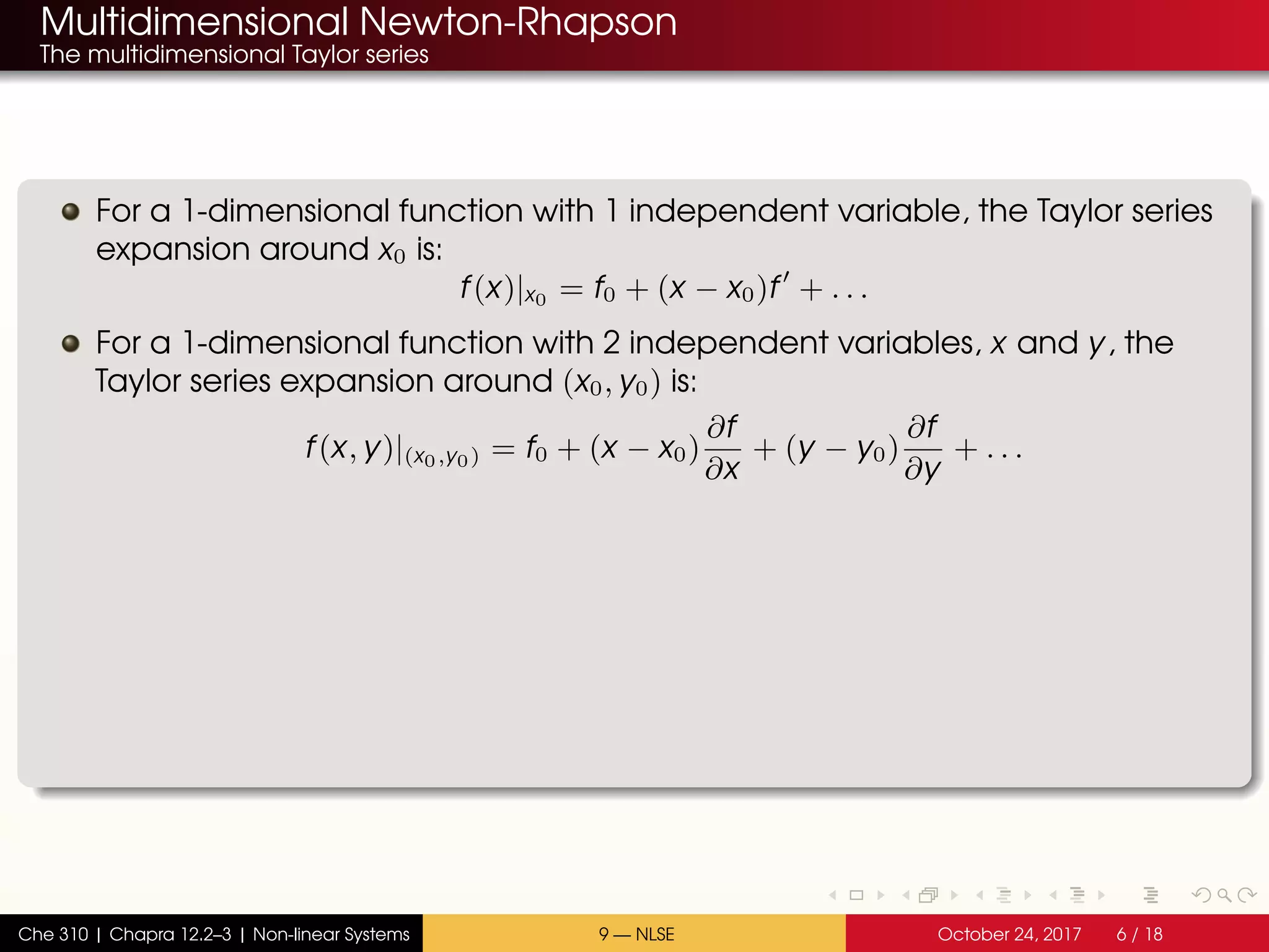
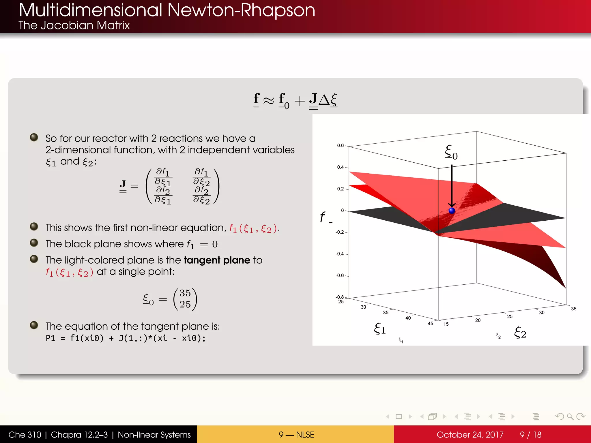
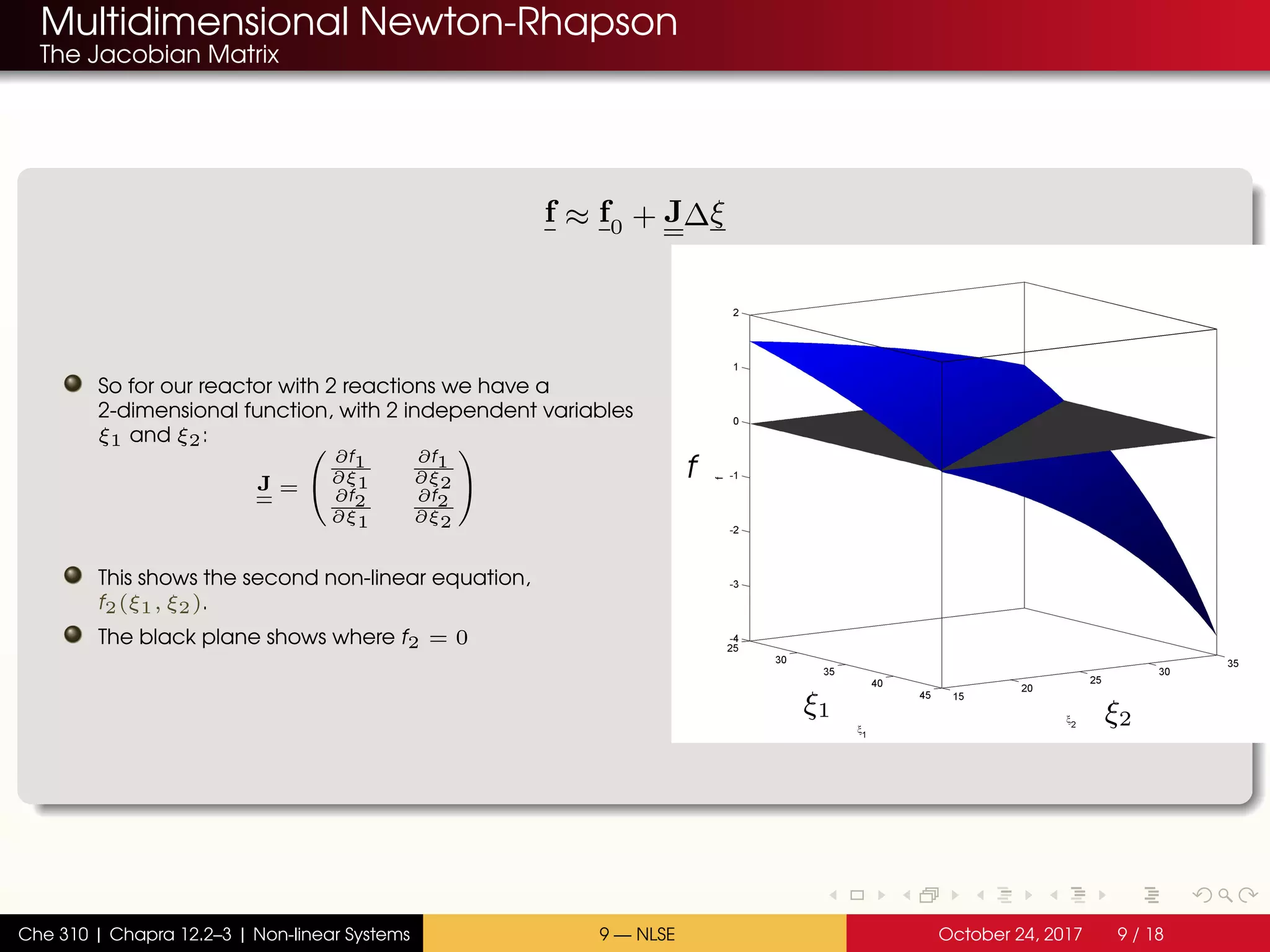
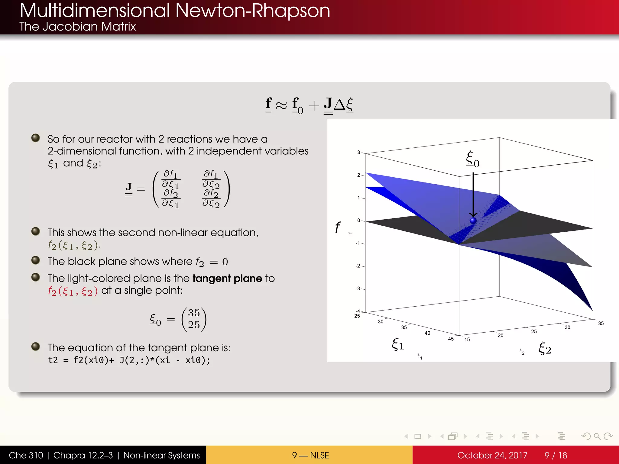
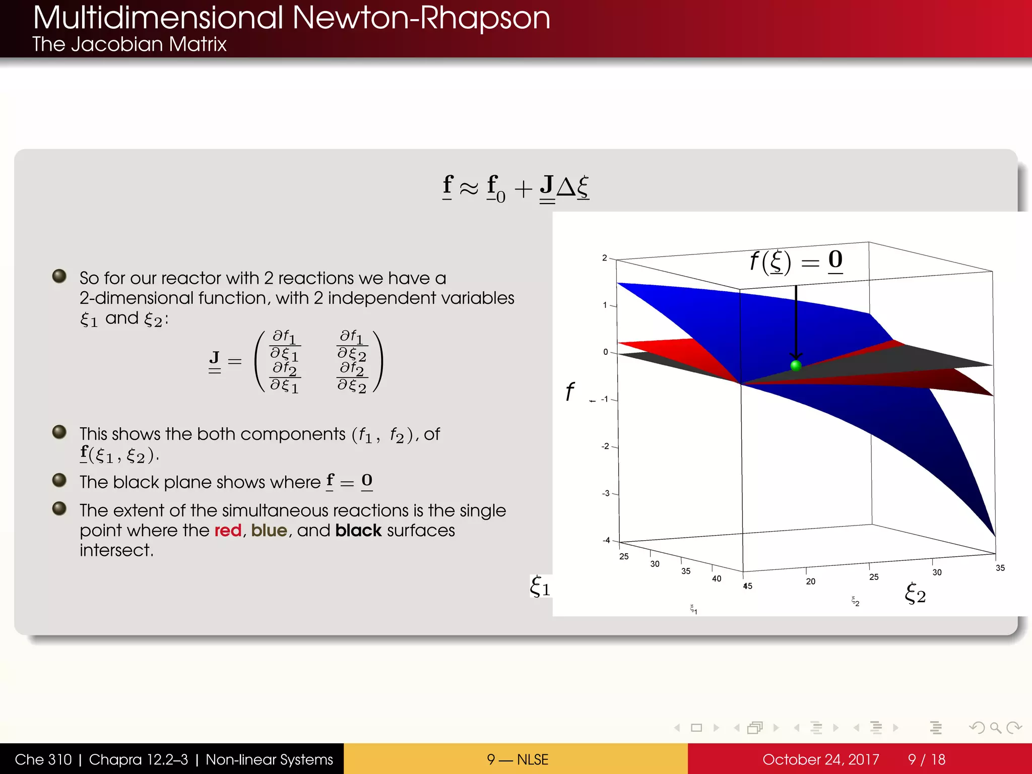
The document discusses solving multiple non-linear equations using the multidimensional Newton-Raphson method. It provides an example of solving for the equilibrium conversion of two coupled chemical reactions. The key steps are: (1) writing the reaction equations in root-finding form as two non-linear equations f1 and f2; (2) defining the Jacobian matrix J with the partial derivatives of f1 and f2; and (3) using the multidimensional Taylor series expansion and Jacobian matrix to linearize the system and iteratively solve for the root where f1 and f2 equal zero.