Downloaded 149 times
![Edited by Foxit Reader
Copyright(C) by Foxit Software Company,2005-2008
For Evaluation Only.
2
x y
1 1
x = y
[ ] 2 , = [ ]
2
x N N N N y N N N N
1 2 3 4 1 2 3 4
x y
x y
3 3
4 4
- In order to approximate strain and stress, the derivatives of shape functions with
respect to coordinate directions are required. Since shape functions depend on s and t
coordinates, chain rule of differentiation must be used.
∂ = ∂ ∂ + ∂ ∂ ∂ = ∂ ∂ + ∂ ∂
∂ ∂ ∂ ∂ ∂ ∂ ∂ ∂ ∂ ∂
i i i , i i i N N x N y N N x N y
s x s y s t x t y t
In the matrix form:
∂ N ∂ x ∂ y ∂ N ∂ N
i i i
∂ ∂ s = s ∂ s ∂ x ∂ x
∂ ≡ [ J
]
N i ∂ x ∂ y ∂ N i ∂ N
i
∂ t ∂ t ∂ t ∂ y ∂ y
where [J] is the Jacobian matrix and its determinant is called the Jacobian. By inverting
the Jacobian matrix, the desired derivatives with respect to x and y can be obtained:
∂ N i ∂ N ∂ y − ∂ y ∂ N
∂ x i i
= −
1 ∂ s = 1
∂ t ∂ s ∂ s
∂ [ J
]
N i ∂ N J
− ∂ x ∂ x ∂ N
i i
∂ y ∂ t ∂ t ∂ s ∂ t
where |J| is the Jacobian (or determinant) and is defined by
= ∂ ∂ − ∂ ∂
∂ ∂ ∂ ∂
x y x y
s t t s
J
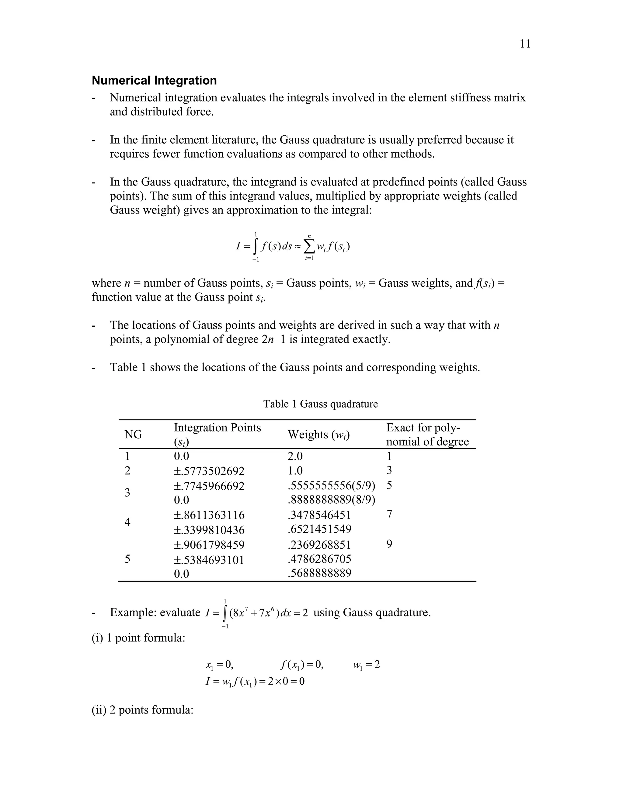
- Since the Jacobian appears in the denominator in the above equation, it must not be
zero anywhere over the domain (–1 s, t 1).
- The mapping is not valid if |J| is zero anywhere over the element.
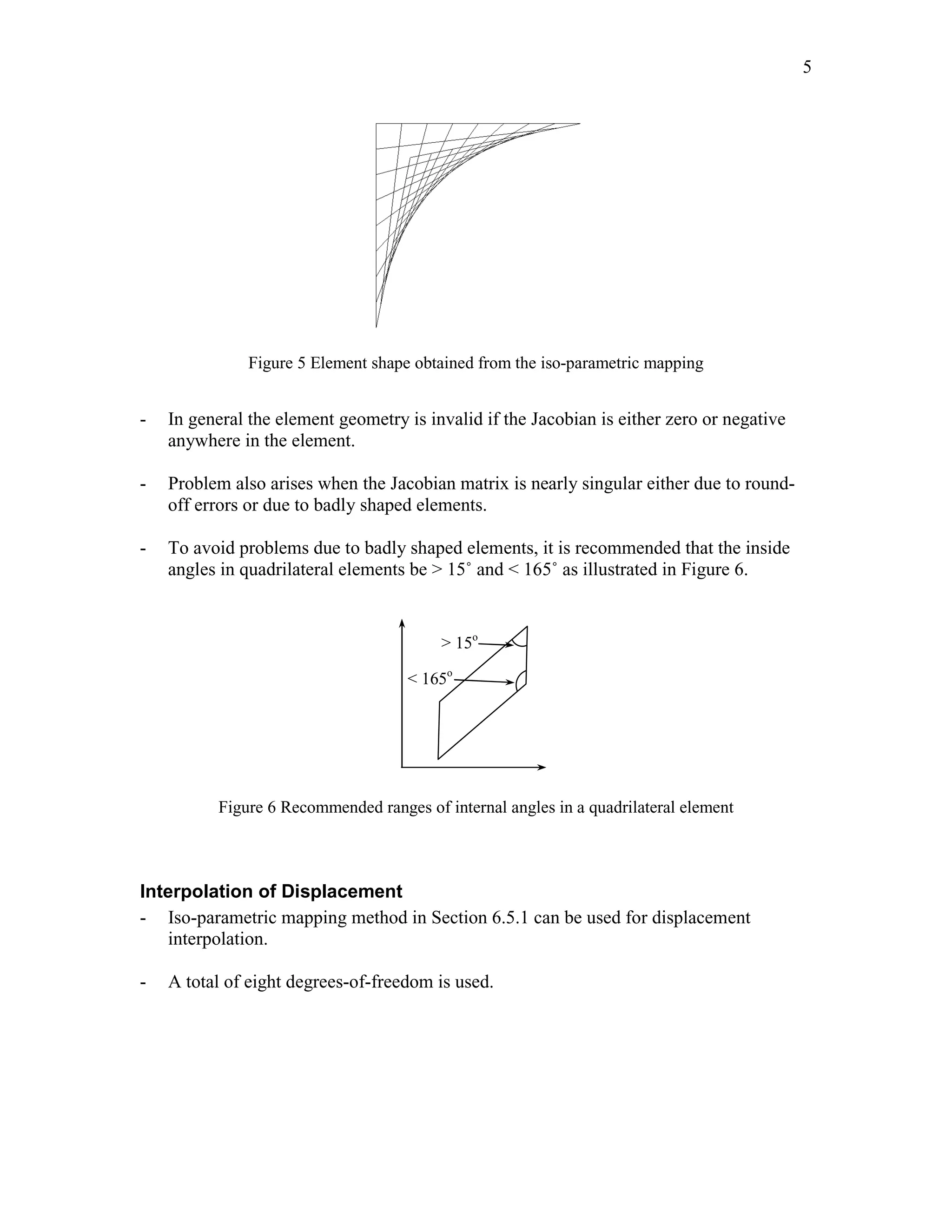
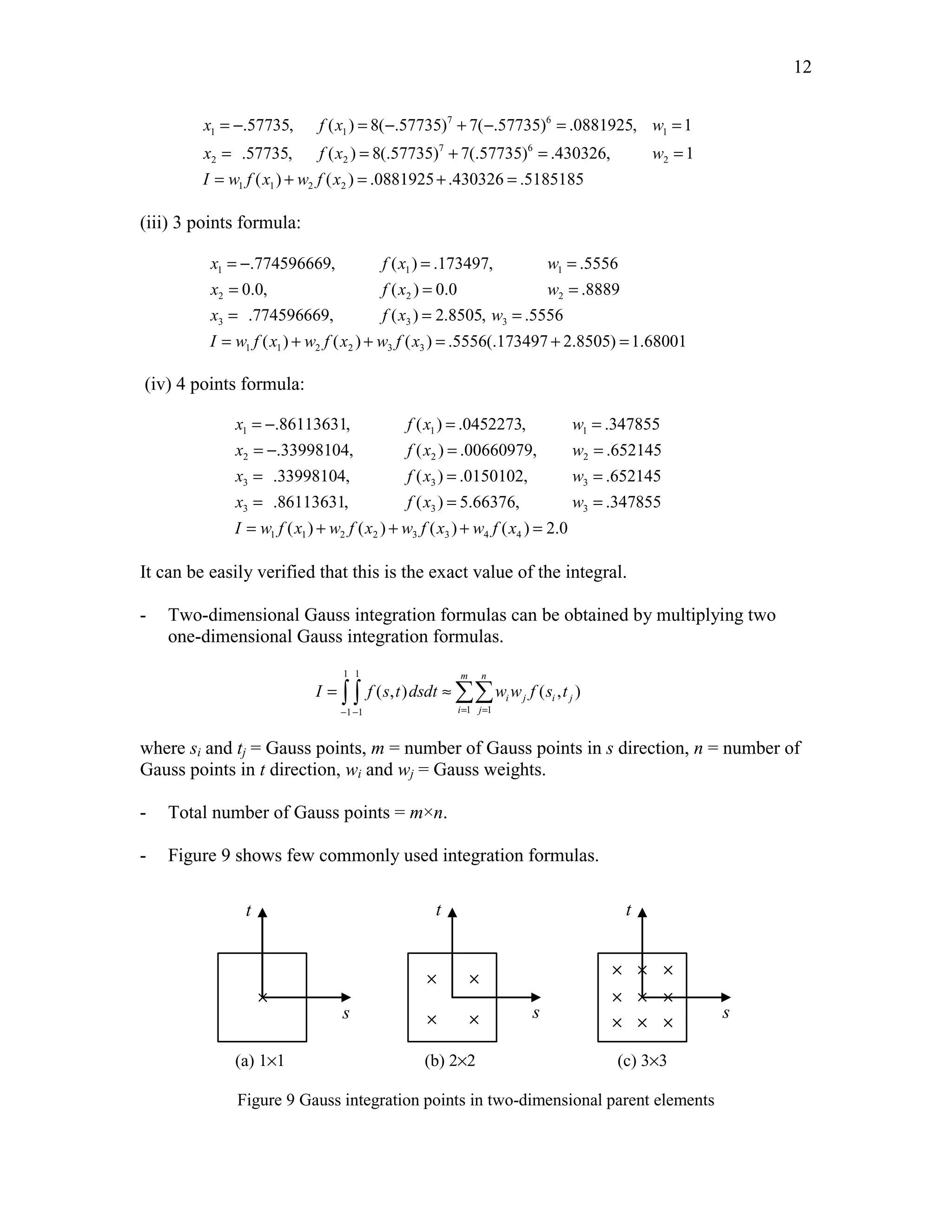
Examples
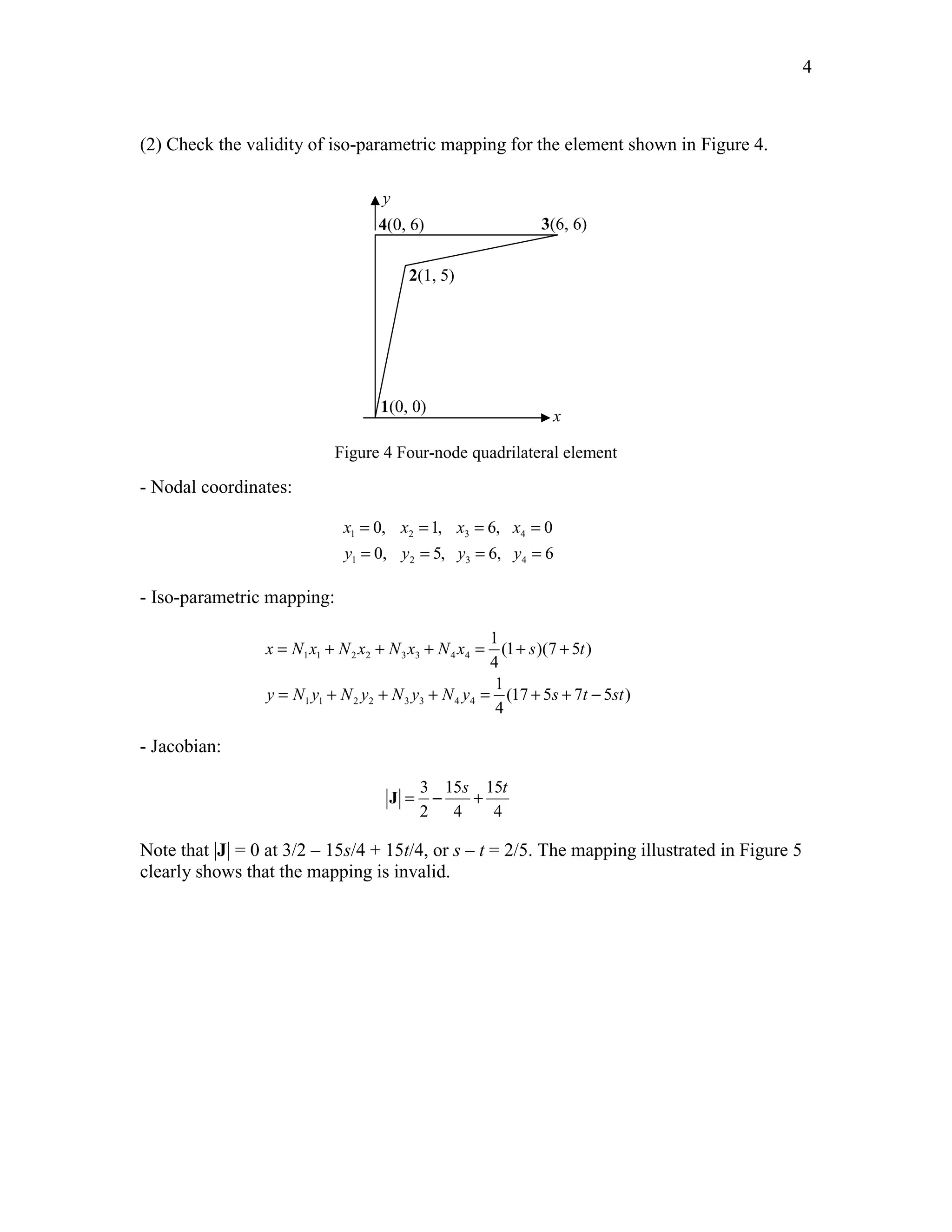
(1) Check the validity of iso-parametric mapping for the element shown in Figure 2
http://swiftmemberreview.com](https://image.slidesharecdn.com/isoparametricmapping-140909111135-phpapp01/75/Isoparametric-mapping-2-2048.jpg)
![Edited by Foxit Reader
Copyright(C) by Foxit Software Company,2005-2008
For Evaluation Only.
3
1(0, 0) 2(1, 0)
3(2, 2)
4(0, 1)
x
y
Figure 2 Four-node quadrilateral element
- Nodal coordinates:
= = = =
= = = =
0, 1, 2, 0
0, 1, 2, 1
x x x x
y y y y
1 2 3 4
1 2 3 4
- Iso-parametric mapping:
= + + + = + = + ++
x N x N x N x N x N N s t st
1 1 2 2 3 3 4 4 2 3
= + + + = + = + + +
y N y N y N y N y N N s t st
1 1 2 2 3 3 4 4 3 4
1
2 (33 )
4
1
2 (3 3 )
4
- Jacobian:
∂ x ∂ y
∂ s ∂ s 1 3 + t 1
+ t
= = ∂ x ∂ y + s + s
∂ t ∂ t
[ ]
4 1 3
J
1 11 1
[(3 )(3 ) (1 )(1 )]
4 28 8
J = + t + s − + t + s = + s + t
Thus, it is clear that |J| > 0 for –1 s 1 and –1 t 1.
Figure 3 Element shape obtained from the iso-parametric mapping
http://swiftmemberreview.com](https://image.slidesharecdn.com/isoparametricmapping-140909111135-phpapp01/75/Isoparametric-mapping-3-2048.jpg)
![Edited by Foxit Reader
Copyright(C) by Foxit Software Company,2005-2008
For Evaluation Only.
6
1
1
2
= 1 2 3 4 2
=
1 2 3 4 3
3
4
4
0 0 0 0
[ ]{ }
0 0 0 0
u
v
u
u N N N N v
v N N N N u
v
u
v
N d
where the same shape functions in geometric interpolation can be used for displacement
interpolation:
= − − 1
= + − 2
3
4
1
(1 )(1 )
4
1
(1 )(1 )
4
1
(1 )(1 )
4
1
(1 )(1 )
4
N s t
N s t
= + +
N s t
N s t
= − +
- Jacobian Matrix
∂ ∂
∂ ∂ ∂ ∂ ∂ ∂ = = −
∂ ∂ ∂ ∂ ∂ ∂
∂ ∂
x y
s s x y x y
x y s t t s
t t
J J
[ ] ,
where
x x
1 1
∂∂ ∂ x = N ∂ N ∂ N ∂ N x 1
x
[ 1 2 3 4 ] 2 = [− 1 + t 1 − t 1 + t − 1 − t
]
2
∂ s ∂ s ∂ s ∂ s s x 4
x
3 3
x x
4 4
1
∂ = − + − − + − 2
∂ 3
4
1
[ 1 1 1 1 ]
4
x
x x
s s s sx
t
x
Similar expressions can be written for derivatives of y with respect to s and t. In general,
the determinant of the Jacobian matrix can be expressed as
http://swiftmemberreview.com](https://image.slidesharecdn.com/isoparametricmapping-140909111135-phpapp01/75/Isoparametric-mapping-6-2048.jpg)
![7
0 1 − t − s + t − 1
+ s y
− 1 + t 0 1
+ s − s − t 1
y
= 1 [ x x x x
]
T
2
8 1 2 3 4
s − t − 1 − s 0 1
+ t y
3
1 − s s + t − 1 − t 0
y
4
J
- Displacement-strain relationship
/
/ 1 0 0 0
/
{ } / 0 0 0 1
/
/ / 01 1 0/
xx
yy
xy
u x
u x
u y
v y
v x
u y v x
v y
ε
ε
γ
∂ ∂
∂ ∂ ∂ ∂ = = ∂ ∂ = ∂ ∂ ∂ ∂ + ∂ ∂ ∂ ∂
ε
∂ u ∂ y − ∂ y ∂ u
∂ x 1
= ∂ t ∂ s ∂ ∂ s
u J
− ∂ x ∂ x ∂ u
∂ y ∂ t ∂ s ∂ t
∂ v ∂ y − ∂ y ∂ v
∂ x 1
= ∂ t ∂ s ∂ ∂ s
v J
− ∂ x ∂ x ∂ v
∂ y ∂ t ∂ s ∂ t
Writing the two equations together:
∂ u / ∂ x ∂ y / ∂ t −∂ y / ∂ s 0 0 ∂ u /
∂ s
∂ u / ∂ y −∂ x / ∂ t ∂ x / ∂ s 0 0 ∂ u /
∂ t
= 1 ∂ v / ∂ x J
0 0 ∂ y / ∂ t −∂ y / ∂ s ∂ v /
∂ s
∂ v / ∂ y 0 0 −∂ x / ∂ t ∂ x / ∂ s ∂ v /
∂ t
The strain can now be expressed as
∂ y / ∂ t −∂ y / ∂ s 0 0 ∂ u / ∂ s ∂ u /
∂ s
ε
1 0 0 0
xx
ε
= 1 −∂ x / ∂ t ∂ x / ∂ s 0 0 ∂ u / ∂ t ∂ u /
∂ t
0 0 0 1 ≡ [ A
]
yy
J
0 0 ∂ y / ∂ t −∂ y / ∂ s ∂ v / ∂ s ∂ v /
∂ s
γ
0 1 1 0
xy
0 0 −∂ x / ∂ t ∂ x / ∂ s ∂ v / ∂ t ∂ v /
∂ t
The derivative of the trial solution with respect to s and t are easy to compute:](https://image.slidesharecdn.com/isoparametricmapping-140909111135-phpapp01/75/Isoparametric-mapping-7-2048.jpg)
![Edited by Foxit Reader
Copyright(C) by Foxit Software Company,2005-2008
For Evaluation Only.
8
1
1
∂ ∂ − + − + − −
2
∂ ∂ − + − − + − ∂ ∂ = 2
≡ − + − + − − 3
∂ ∂ − + − − + − 3
4
4
/ 1 0 1 0 1 0 1 0
/ 1 1 0 1 0 1 0 1 0
[ ]{ }
/ 4 0 1 0 1 0 1 0 1
/ 0 1 0 1 0 1 0 1
u
v
u s t t t t u
u t s s s s v
v s t t t t u
v t s s s s v
u
v
G d
The displacement-strain matrix [B] can now be written as follows:
/
/
[ ] [ ][ ]{ } [ ]{ }
/
/
xx
yy
xy
u s
u t
v s
v t
ε
ε
γ
∂ ∂
∂ ∂ = = ≡ ∂ ∂
∂ ∂
A AG d B d
- The displacement-strain matrix [B] is not constant. Thus, the value of strain and
stress within an element changes as a function of position.
Finite Element Matrix Equation
- The element stiffness matrix is:
1 1
k = ∫∫ B C B ≡ ∫ ∫ B C B J (0.1)
[ ] [ ]T [ ][ ] [ ]T [ ][ ]
h dA h dsdt
1 1
A
− −
- Different from the triangular element, the element stiffness matrix is not constant
within an element. Thus, analytical integration is not trivial. Numerical integration
ethod using Gaussian quadrature will be discussed in the next section.
- Work done by concentrated forces:
NF x y x y x y x y NF W = F u + F v + F u + F v + F u + F v + F u + F v ≡ d Q
1 1 1 1 2 2 2 2 3 3 3 3 4 4 4 4 { }T{ }
NF x y x y x y x y Q = F F F F F F F F is the vector of applied nodal
where 1 1 2 2 3 3 4 4 { } [ ]T
forces.
- Work done by distributed load:
W = d h∫ N T dS = d Q
{ }T [ ]T{ } { }T{ }
T T
S
http://swiftmemberreview.com](https://image.slidesharecdn.com/isoparametricmapping-140909111135-phpapp01/75/Isoparametric-mapping-8-2048.jpg)
![Edited by Foxit Reader
Copyright(C) by Foxit Software Company,2005-2008
For Evaluation Only.
9
4
1
3
2
4
3
1 2
s
s
s
s
S
S
S
S
Tx
Ty
Figure 7 Coordinates for evaluation of boundary integrals
Side 1-2:
(1 − s ) / 2 0 (1 + s
) / 2 0 0 0 0 0
= − + − ≤ ≤
[ ] , 1 1
0 (1 )/2 0 (1 )/2 0 0 0 0
s
s s
N
Side 2-3:
0 0 (1 − s ) / 2 0 (1 + s
) / 2 0 0 0
= − ≤ ≤ − +
[ ] , 1 1
0 0 0 (1 )/2 0 (1 )/2 0 0
s
s s
N
Side 3-4:
0 0 0 0 (1 − s )/2 0 (1 + s
)/2 0
= − + − ≤ ≤
[ ] , 1 1
0 0 0 0 0 (1 )/2 0 (1 )/2
s
s s
N
Side 4-1:
(1 + s )/2 0 0 0 0 0 (1 − s
)/2 0
= + − − ≤ ≤
[ ] , 1 1
0 (1 )/2 0 0 0 0 0 (1 )/2
s
s s
N
- As an example, consider side 2-3, as shown in Figure 7. The iso-parametric
mapping for side 2-3 is
1 − s 1 + s 1 − s 1
+
s
x = x + x ,
y = y + y
2 3 2 3
2 2 2 2
dx x x x x
3 2 3 2
1 1
x x dx ds
2 3
or
2 2 2 2
ds
dy y y y y
3 2 3 2
or
dy ds
2 2
ds
= − + = − = −
= − = −
The Jacobian of the transformation from S to s is defined as
side2-3
dS
J
ds
=
with reference to Figure 8 it can be developed as follows. From geometry
http://swiftmemberreview.com](https://image.slidesharecdn.com/isoparametricmapping-140909111135-phpapp01/75/Isoparametric-mapping-9-2048.jpg)
![10
-1
(x2, y2)
1
s
(x3, y3)
dx
dy
S
dS
Side 2-3 of parent element
Figure 8 Evaluation of work done by applied pressure along side 2-3
1 1
dS = dx 2 + dy 2 = ( x − x ) 2 + ( y − y )
2
ds = L ds
3 2 3 2 23
2 2
Thus, the Jacobian for each side is equal to half the length of that side. Thus,
−
1 1
− = T = T = x
+
,side 2-3 23 23
side 2 3 1 1
0 0
0 0
(1 ) / 2 0
1 0 (1 ) / 2 1
{ } [ ] { } [ ] { }
2 (1 ) / 2 0 2
0 (1 )/2
0 0
0 0
T
y
s
s T
h dS h L ds h L ds
s T
s
− − −
+
Q ∫ N T ∫ N T ∫
Carrying out the integration gives
hL
Q = 23
T T T T
,side2-3 { } [0 0 0 0]
2
T
T x y x y
- Similar to the linear triangular element, this equation says that total pressure along a
side is divided equally among the two nodes along the side.
- All quantities needed for the potential energy have now been expressed in terms of
nodal unknowns. From the principle of minimum total potential energy,
[ ]{ } { } NT T k d = Q +Q
where [k] is 8×8 element stiffness matrix, {d} is 8×1 nodal displacement vector, and
{QNT+QT} is 8×1 applied nodal force vector.](https://image.slidesharecdn.com/isoparametricmapping-140909111135-phpapp01/75/Isoparametric-mapping-10-2048.jpg)
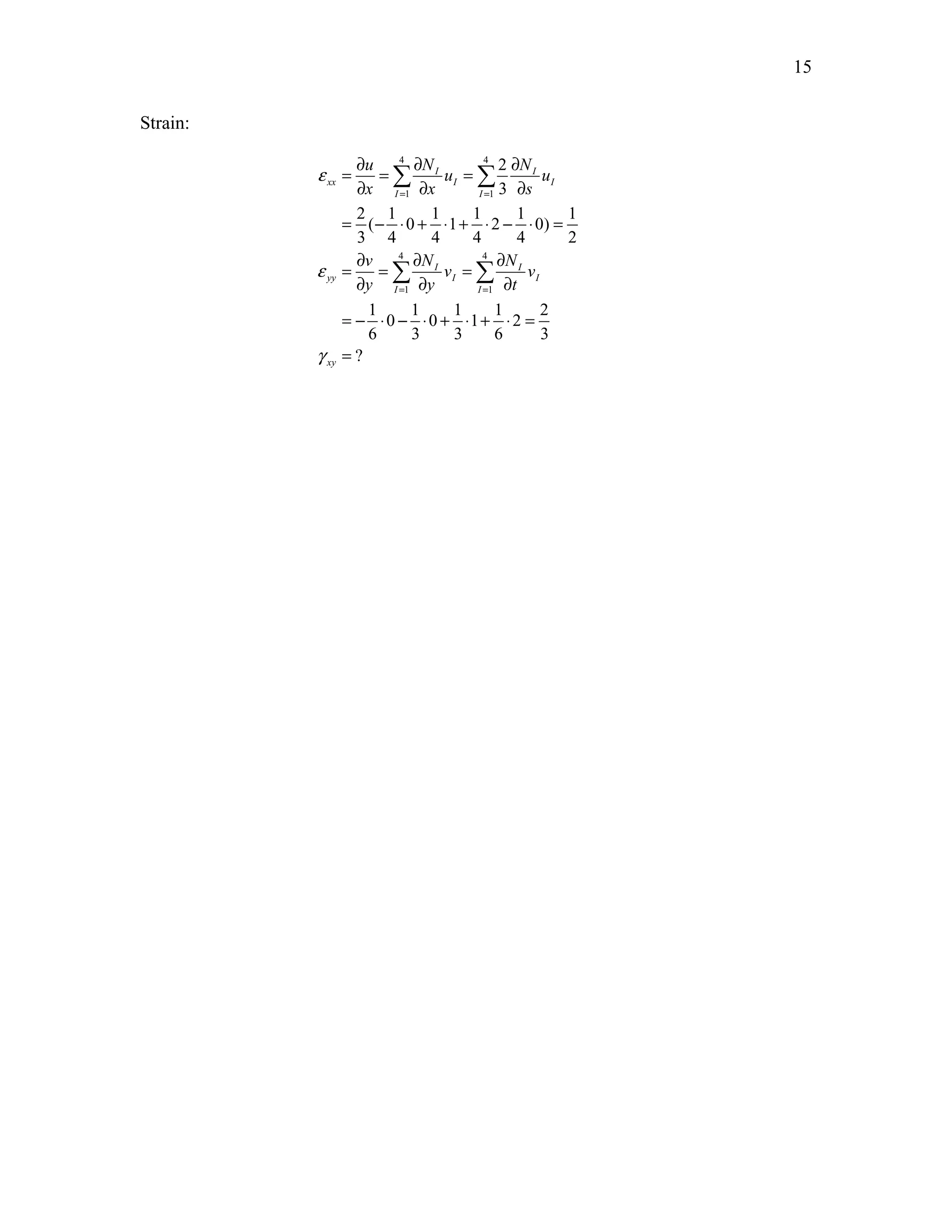
![13
- The element stiffness matrix can be evaluated using 2×2 Gauss integration formulas:
1 1 2 2
k = ∫ ∫ B C B J ≈ ΣΣ B C B J
[ ] [ ][ ][ ]T [ ( , )][ ][ ( , )]T ( , )
h dsdt h ww s t s t s t
− 1 − 1 = 1 =
1
i j i j i j i j
i j
Example: Interpolation using Quadrilateral Element
For a rectangular element shown in the figure, displacements at four nodes are given
by {u1, v1, u2, v2, u3, v3, u4, v4} = {0.0, 0.0, 1.0, 0.0, 2.0, 1.0, 0.0, 2.0}. Calculate
displacement and strain at point (s, t) = (1/3, 0).
x
y
4 (0,2) 3 (3,2)
1 (0,0) 2 (3,0)
s
t
4 (-1,1) 3 (1,1)
1 (-1,-1) 2 (1,-1)
First, the shape functions are given in the parent element as
= − − = + −
= + + = − +
1 1
(1 )(1 ), (1 )(1 )
4 4
1 1
(1 )(1 ), (1 )(1 )
4 4
N s t N s t
1 2
N s t N s t
3 4
Especially when (s, t) = (1/3, 0),
1 1 1 1
, , ,
6 3 3 6
N = N = N = N =
1 2 3 4
Interpolation of geometry [find physical coordinates corresponding to (s, t) = (1/3, 0)]:
4
x Σ
Nx
1
4
y = Ny
= ⋅ + ⋅ + ⋅ + ⋅ = 1
1 1 1 1
0 3 3 0 2
6 3 3 6
1 1 1 1
0 0 2 2 1
6 3 3 6
I I
I
I I
I
=
=
= = ⋅ + ⋅ + ⋅ + ⋅ =
Σ
Displacement interpolation (Same shape function for geometry interpolation: Iso-parametric)](https://image.slidesharecdn.com/isoparametricmapping-140909111135-phpapp01/75/Isoparametric-mapping-13-2048.jpg)
![14
Σ
4
u = Nu
= ⋅ + ⋅ + ⋅ + ⋅ = 1
v = Σ
4
Nv
= ⋅ + ⋅ + ⋅ + ⋅ = 1
1 1 1 1
0 1 2 0 1
6 3 3 6
1 1 1 1 2
0 0 1 2
6 3 3 6 3
I I
I
I I
I
=
=
Derivatives of shape functions (Note shape functions depend on s and t):
∂ = − − = − ∂ = − − = − ∂ ∂
∂ = − = ∂ = − + = − ∂ ∂
∂ ∂ = + = = + =
∂ ∂
∂ ∂ = − + = − = − = ∂ ∂
1 1 1 1
(1 ) (1 )
4 4 4 6
1 1 1 1
(1 ) (1 )
4 4 4 3
1 1 1 1
(1 ) (1 )
4 4 4 3
1 1 1 1
N N
1 1
t s
s t
N N
2 2
t s
s t
N N
3 3
t s
s t
N N
4 4
(1 t ) (1 s
)
4 4 4 6
s t
Jacobian matrix:
∂ = − ⋅ + ⋅ + ⋅ − ⋅ = ∂
∂ = − ⋅ + ⋅ + ⋅ − ⋅ = ∂
∂ =− ⋅ − ⋅ + ⋅ + ⋅ =
∂
∂ = − ⋅ − ⋅ + ⋅ + ⋅ = ∂
1 1 1 1 3
0 3 3 0
4 4 4 4 2
1 1 1 1
0 0 2 2 0
4 4 4 4
1 1 1 1
0 3 3 0 0
6 3 3 6
1 1 1 1
0 0 2 2 1
6 3 3 6
x
s
y
s
x
t
y
t
∂ ∂ 3 2
0 0
= ∂ ∂ = 1
= ∂ ∂ ∂ ∂
[ ] 2 , [ ] 3
0 1 0 1
x y
s s
x y
t t
−
J J
Derivative of shape functions:
∂ N = ∂ N ∂ x + ∂ N ∂ y I I I ∂ ⇒ N ∂ N
I I
∂ s ∂ x ∂ s ∂ y ∂ s ∂ s = ∂ x
[ J
]
∂ N = ∂ N ∂ x + ∂ N ∂ y ∂ N ∂ N
I I I I I
∂ t ∂ x ∂ t ∂ y ∂ t ∂ t ∂ y
∂ N I ∂ N ∂ N 2
∂ N
I ∂ x 2
0 I I
= ∂ [ J
] −
1
∂ s = ∂ ∂ ∂ 3
s = 3 s
N I N ∂ N I 0 1
I ∂ N
I
∂ y ∂ t ∂ t ∂ t
](https://image.slidesharecdn.com/isoparametricmapping-140909111135-phpapp01/75/Isoparametric-mapping-14-2048.jpg)

The document provides an in-depth analysis of the four-node iso-parametric quadrilateral element used in finite element analysis, detailing its characteristics such as eight unknowns (displacements at each node) and the iso-parametric mapping process between physical and reference elements. It discusses the importance of the Jacobian matrix in ensuring valid mappings and highlights potential issues arising from singular or poorly-shaped elements. Additionally, it emphasizes the recommended angular range for quadrilateral elements to maintain geometric accuracy.
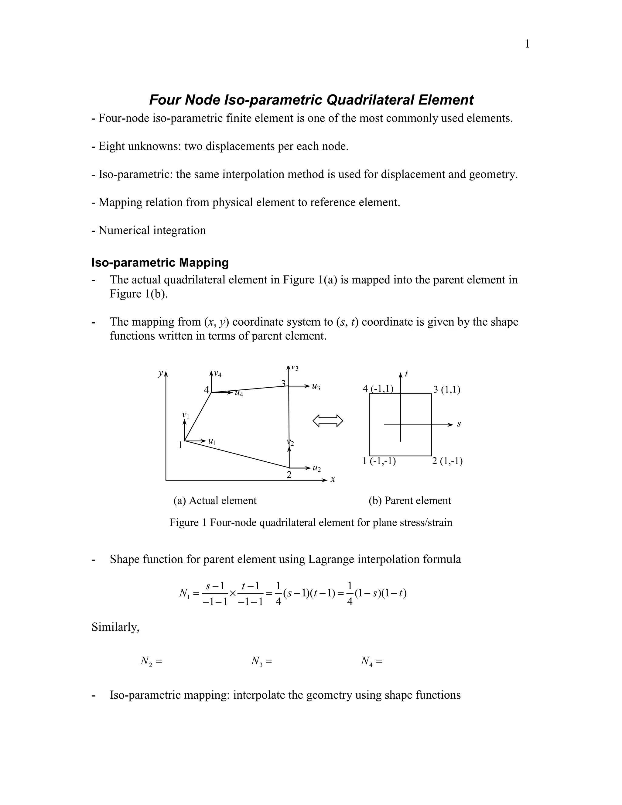
Introduction to the four-node iso-parametric quadrilateral element, interpolation methods, shape functions, and mapping from physical to reference element.
Details on the use of shape function derivatives, the Jacobian matrix for coordinate transformation, and conditions for valid iso-parametric mapping.
Examples of nodal coordinates for iso-parametric mapping and conditions for maintaining validity in mapping using Jacobians.
Implications of Jacobian values on element geometry, specifying acceptable angle ranges to prevent invalid mapping.
Introduction to interpolation of displacements with shape functions, reference to Jacobian and displacement-strain relationships through matrix forms.
Details on deriving stiffness matrices, work done by forces, and boundary evaluation within finite element analysis.
Introduction to numerical integration, specific focus on Gauss quadrature, its advantages, and mathematical implementation.
Discussion on calculating element stiffness matrix using Gauss integration, and examples of displacement and strain interpolation.