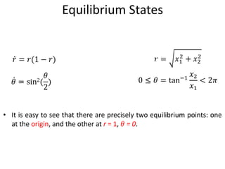
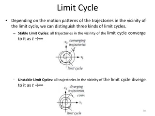
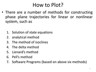
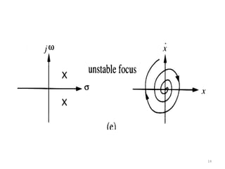
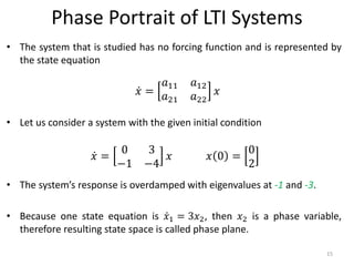
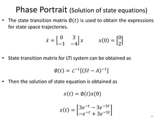
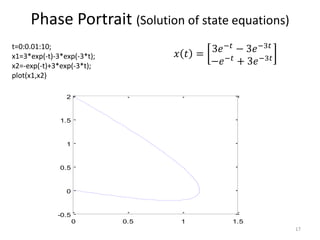
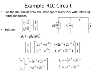
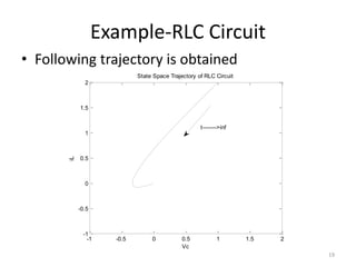
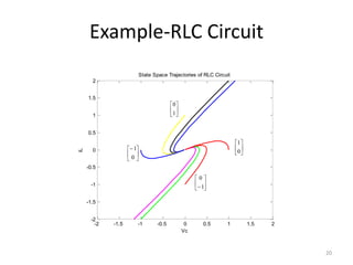
The document discusses phase plane analysis, which is a graphical method to visualize the behavior of nonlinear systems by plotting trajectories in the phase plane defined by the state variables. It provides examples of analyzing linear time-invariant systems by plotting trajectories based on the state equations. The document also discusses concepts like equilibrium points, singular points, and limit cycles that can occur for nonlinear systems through phase plane analysis.

1. Modern Control Systems (MCS)
Dr. Imtiaz Hussain
Assistant Professor
email: imtiaz.hussain@faculty.muet.edu.pk
URL :http://imtiazhussainkalwar.weebly.com/
Lecture-7
Phase Plane Analysis
1

2. Introduction
• The definition for stability for LTI systems is an
easy concept to understand (eigenvalues).
• It is necessary to extend the concept of
stability to nonlinear systems.
2

3. • To generate motion trajectories corresponding to
various initial conditions in the phase plane.
• To examine the qualitative features of the trajectories.
• In such a way, information concerning stability and
other motion patterns of the system can be obtained.
Basic Idea
3

4. State Space Trajectories
• The unforced response of a system released from any
initial point x(to) traces a curve or trajectory in state
space, with time t as an implicit function along the
trajectory.
• When state variables are represented as phase
variables, the state space is called phase space or
phase plane.
• The family of all trajectories (which started by different
initial points) is called phase portrait.
4

5. • A graphical method: to visualize what goes on
in a nonlinear system without solving the
nonlinear equations analytically.
• 2. Limitation: limited for second-order (or
first –order) dynamic system; however, some
practical control systems can be approximated
as second-order systems.
Phase Plane Analysis
5

6. How to Plot?
• There are a number of methods for constructing
phase plane trajectories for linear or nonlinear
system, such as
1. Solution of state equations
2. analytical method
3. The method of isoclines
4. The delta method
5. Lienard’s method
6. Pell’s method
7. Software Programs (based on above six methods)
6

7. Phase Plane Analysis of Linear
Systems
7

8. - Consider the second-order linear system
is the general solution
• Where the eigenvalues and are the solutions
of the characteristic equation
0
x ax bx
  
1 2
1 2
( ) t t
x t k e k e
 
 
1
 2

2
1 2
2 2
1 2
( )( ) 0
( 4 ) ( 4 )
,
2 2
s as b s s
a a b a a b
 
 
     
     
  
8

9. There is only one singular point (assuming
), namely the origin.
1. and are both real and have the same sign
(positive or negative)
2. and are both real and have opposite
signs (saddle point)
3. and are complex conjugate with non-zero
real parts
4. and are complex conjugates with real
parts equal to zero (center point)
1
 2

1
 2

1
 2

1
 2

0
b 
9

10. 10

11. 11

12. 12

13. 13

14. 14

15. Phase Portrait of LTI Systems
• The system that is studied has no forcing function and is represented by
the state equation
• Let us consider a system with the given initial condition
• The system’s response is overdamped with eigenvalues at -1 and -3.
• Because one state equation is 𝑥1 = 3𝑥2, then 𝑥2 is a phase variable,
therefore resulting state space is called phase plane.
15
𝑥 =
𝑎11 𝑎12
𝑎21 𝑎22
𝑥
𝑥 =
0 3
−1 −4
𝑥 𝑥 0 =
0
2

16. Phase Portrait (Solution of state equations)
• The state transition matrix ∅(𝑡) is used to obtain the expressions
for state space trajectories.
• State transition matrix for LTI system can be obtained as
• Then the solution of state equation is obtained as
16
𝑥 =
0 3
−1 −4
𝑥 𝑥 0 =
0
2
𝑥 𝑡 = ∅ 𝑡 𝑥(0)
∅ 𝑡 = L−1 𝑆𝐼 − 𝐴 −1
𝑥 𝑡 = 3𝑒−𝑡 − 3𝑒−3𝑡
−𝑒−𝑡 + 3𝑒−3𝑡

17. Phase Portrait (Solution of state equations)
17
𝑥 𝑡 = 3𝑒−𝑡
− 3𝑒−3𝑡
−𝑒−𝑡
+ 3𝑒−3𝑡
t=0:0.01:10;
x1=3*exp(-t)-3*exp(-3*t);
x2=-exp(-t)+3*exp(-3*t);
plot(x1,x2)
0 0.5 1 1.5
-0.5
0
0.5
1
1.5
2

18. Example-RLC Circuit
• For the RLC circuit draw the state space trajectory with following
initial conditions.
• Solution













2
1
0
0
)
(
)
(
L
c
i
v

































2
1
)
2
(
)
(
)
2
2
(
)
2
(
2
2
2
2
t
t
t
t
t
t
t
t
L
c
e
e
e
e
e
e
e
e
i
v
)
(
)
(
)
( 0
x
t
t
x 






















t
t
t
t
L
c
e
e
e
e
i
v
2
2
3
3
3
t
t
L
t
t
c
e
e
i
e
e
v
2
2
3
3
3










Vc
+
-
+
-
18

19. Example-RLC Circuit
• Following trajectory is obtained
-1 -0.5 0 0.5 1 1.5 2
-1
-0.5
0
0.5
1
1.5
2
Vc
iL
State Space Trajectory of RLC Circuit
t-------->inf
19

20. Example-RLC Circuit
-2 -1.5 -1 -0.5 0 0.5 1 1.5 2
-2
-1.5
-1
-0.5
0
0.5
1
1.5
2
Vc
iL
State Space Trajectories of RLC Circuit






0
1 





0
1






1
0






1
0
20

21. • Equilibrium point is defined as a point where the
system states can stay forever
• This implies that
• A singular point is an equilibrium point in the phase
plane.
0

)
(t
x

Equilibrium Point and Singular Points
21

22. Equilibrium Point
• The equilibrium or stationary state of the system
is when
0

)
(t
x

-2 -1.5 -1 -0.5 0 0.5 1 1.5 2
-2
-1.5
-1
-0.5
0
0.5
1
1.5
2
Vc
iL
State Space Trajectories of RLC Circuit
22

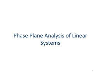
23. Examples of LTI systems
23
1.
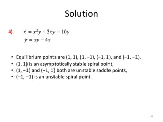
𝑥1
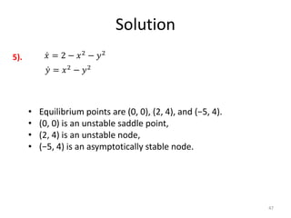
𝑥2
=
0 1
−1 −4
𝑥1
𝑥2
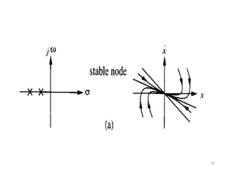
(overdamped Stable System, [stable node])
2.
𝑥1
𝑥2
=
0 1
2 −5
𝑥1
𝑥2
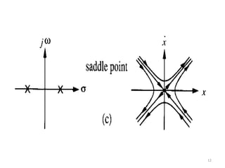
(overdamped unstable [saddle point]
3.
𝑥1
𝑥2
=
0 1
−4 −1
𝑥1
𝑥2
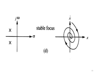
(underdamped stable System, stable focus)
4.
𝑥1
𝑥2
=
0 1
−10 4
𝑥1
𝑥2
(underdamped Unstable System, unstable focus)
5.
𝑥1
𝑥2
=
0 1
−1 6
𝑥1
𝑥2
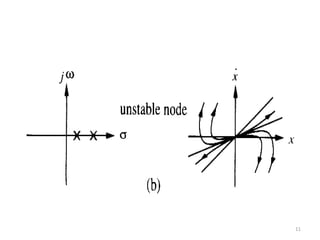
(overdamped Unstable System, [unstable node])

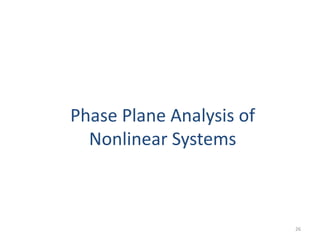
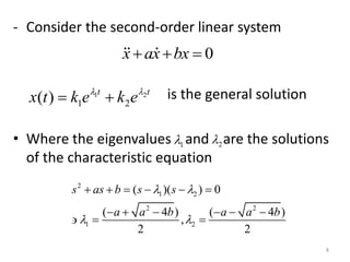
24. Software Solution
24
x1dom = linspace(-5,5,51);
x2dom = linspace(-5,5,51);
[x1,x2] = meshgrid(xdom,ydom); % generate mesh of domain
x1dot = x1; % dx1/dt
X2dot= = -x1-4*x2; % dx2/dt
quiver(x1,x2,x1dot,x2dot) % velocity Vectors
𝑥1
𝑥2
=
0 1
−1 −4
𝑥1
𝑥2

25. Enter Equations in PPlane Applet
25

26. Phase Plane Analysis of
Nonlinear Systems
26

27. Introduction
• In discussing the phase plane analysis of
nonlinear systems, two points should be kept in
mind:
– Phase plane analysis of nonlinear systems is related
to that of liner systems, because the local behavior
of nonlinear systems can be approximated by the
behavior of a linear system.
– Nonlinear systems can display much more
complicated patterns in the phase plane, such as
multiple equilibrium points and limit cycles.
27

28. Example
• Consider the second-order system with state variables 𝑥1 and 𝑥2
whose dynamics are most easily described in polar coordinates via
the equations
• Where the radius r is given as
• And the angle θ is
𝑟 = 𝑟(1 − 𝑟)
𝜃 = sin2(
𝜃
2
)
𝑟 = 𝑥1
2
+ 𝑥2
2
0 ≤ 𝜃 = tan−1
𝑥2
𝑥1
< 2𝜋

29. Equilibrium States
• It is easy to see that there are precisely two equilibrium points: one
at the origin, and the other at r = 1, 𝜃 = 0.
𝑟 = 𝑟(1 − 𝑟)
𝜃 = sin2(
𝜃
2
)
𝑟 = 𝑥1
2
+ 𝑥2
2
0 ≤ 𝜃 = tan−1
𝑥2
𝑥1
< 2𝜋

30. Example: Simple Pendulum
• Consider the pendulum shown in
figure.
𝑀𝐿2𝜃 + 𝑏𝜃 + 𝑀𝑔𝐿 sin 𝜃 = 0
Where,
L: the pendulum’s length
M: its mass
b: the friction coefficient at the hinge
g: the gravity constant.

31. • Letting
𝑥1 = 𝜃 and 𝑥2 = 𝜃
1 2
x x

2 2 1
2
sin
b g
x x x
MR R
  
𝑀𝐿2
𝜃 + 𝑏𝜃 + 𝑀𝑔𝐿 sin 𝜃 = 0
Example: Simple Pendulum
• State equation of the system are given as

32. • The equilibrium points:
x2 = 0, sin x1 = 0
(0, 0) and (π, 0)
• The pendulum resting exactly at the vertical up and
down positions.
1 2
x x
 2 2 1
2
sin
b g
x x x
MR R
  

33. Example
• Consider a nonlinear system described by
following state equations determine the
number of equilibrium point(s) of the system.
33
𝑥 = 𝑥 − 𝑦
𝑦 = 𝑥2 + 𝑦2 − 2
Answer
(1, 1) and (−1, −1).

34. Example
• Consider a nonlinear system described by
following state equations determine the
number of equilibrium point(s) of the system.
34
𝑥 = 𝑥 − 𝑥𝑦
𝑦 = 𝑦 + 2𝑥𝑦
Answer
(0, 0) and (−1/2, 1).

35. Local Behavior of Nonlinear Systems
• If the singular point of interest is not at the origin, by
defining the difference between the original state and the
singular point as a new set of state variables, we can shift
the singular point to the origin.
• Using Taylor expansion a second order nonlinear system can
be rewritten in the form
35
𝑥1 = 𝑎𝑥1 + 𝑏𝑥2 + 𝑔(𝑥1, 𝑥2)
𝑥2 = 𝑐𝑥1 + 𝑑𝑥2 + ℎ(𝑥1, 𝑥2)

36. Local Behavior of Nonlinear Systems
• In the vicinity of the origin, the higher order terms can be
neglected, and therefore, the nonlinear system trajectories
essentially satisfy the linearized equation
• As a result, the local behavior of the nonlinear system
can be approximated by the patterns shown by linear
systems
36
𝑥1 = 𝑎𝑥1 + 𝑏𝑥2
𝑥2 = 𝑐𝑥1 + 𝑑𝑥2

37. Limit Cycle
• In the phase plane, a limit cycle is defied as an isolated
closed curve.
• The trajectory has to be both closed, indicating the
periodic nature of the motion, and isolated, indicating the
limiting nature of the cycle (with near by trajectories
converging or diverging from it).
37

38. Limit Cycle
• Depending on the motion patterns of the trajectories in the vicinity of
the limit cycle, we can distinguish three kinds of limit cycles.
– Stable Limit Cycles: all trajectories in the vicinity of the limit cycle converge
to it as t →∞
– Unstable Limit Cycles: all trajectories in the vicinity of the limit cycle diverge
to it as t →∞
38

39. Limit Cycle
– Semi-Stable Limit Cycles: some of the trajectories in the vicinity of the limit
cycle converge to it as t →∞
39

40. Example
• Find the equilibrium point(s) of the nonlinear
system. Then determine the type and stability of
each equilibrium point.
• If system exhibits limit cycles then determine
the nature of limit cycle as well.
40
𝑥 = 𝑦 − 𝑥(𝑥2 + 𝑦2 − 1)
𝑦 = −𝑥 − 𝑦(𝑥2 + 𝑦2 − 1)

41. Example
• Find the equilibrium point(s) of each nonlinear
system given below. Then determine the type
and stability of each equilibrium point.
• If system exhibits limit cycles then determine
the nature of limit cycle as well.
41
𝑥 = 𝑦 + 𝑥(𝑥2
+ 𝑦2
− 1)
𝑦 = −𝑥 + 𝑦(𝑥2 + 𝑦2 − 1)
𝑥 = 𝑦 − 𝑥(𝑥2
+ 𝑦2
− 1)2
𝑦 = −𝑥 − 𝑦(𝑥2 + 𝑦2 − 1)2
1). 2).

42. Exercise
42
𝑥 = 𝑥𝑦 − 3𝑦
𝑦 = 𝑥𝑦 − 3𝑥
1).
𝑥 = 𝑥2 − 3𝑥𝑦 + 2𝑥
𝑦 = 𝑥 + 𝑦 − 1
2).
𝑥 = 𝑥2 + 𝑦2 − 13
𝑦 = 𝑥𝑦 − 2𝑥 − 2𝑦 + 4
3).
𝑥 = 𝑥2𝑦 + 3𝑥𝑦 − 10𝑦
𝑦 = 𝑥𝑦 − 4𝑥
4).
𝑥 = 2 − 𝑥2
− 𝑦2
𝑦 = 𝑥2 − 𝑦2
5).
• Find the equilibrium point(s) of each nonlinear system given
below. Then determine the type and stability of each
equilibrium point. If system exhibits limit cycles then determine
the nature of limit cycle as well.

43. Solution
43
𝑥 = 𝑥𝑦 − 3𝑦
𝑦 = 𝑥𝑦 − 3𝑥
1).
• Equilibrium points are (0, 0) and (−3, 3).
• (0, 0) is a stable center,
• (−3, 3) is an unstable saddle point.

44. Solution
44
𝑥 = 𝑥2
− 3𝑥𝑦 + 2𝑥
𝑦 = 𝑥 + 𝑦 − 1
2).
• Equilibrium points are (0, 1) and (1/4, 3/4)
• (0, 1) is an unstable saddle point,
• (1/4, 3/4) is an unstable spiral point.

45. Solution
45
𝑥 = 𝑥2
+ 𝑦2
− 13
𝑦 = 𝑥𝑦 − 2𝑥 − 2𝑦 + 4
3).
• Equilibrium points are (2, 3), (2, −3), (3, 2) and (−3, 2).
• (2, 3) is an unstable saddle point
• (2, −3) is an unstable saddle point
• (3, 2) is an unstable node,
• (−3, 2) is an asymptotically stable node.

46. Solution
46
𝑥 = 𝑥2
𝑦 + 3𝑥𝑦 − 10𝑦
𝑦 = 𝑥𝑦 − 4𝑥
4).
• Equilibrium points are (1, 1), (1, −1), (−1, 1), and (−1, −1).
• (1, 1) is an asymptotically stable spiral point,
• (1, −1) and (−1, 1) both are unstable saddle points,
• (−1, −1) is an unstable spiral point.

47. Solution
47
𝑥 = 2 − 𝑥2
− 𝑦2
𝑦 = 𝑥2
− 𝑦2
5).
• Equilibrium points are (0, 0), (2, 4), and (−5, 4).
• (0, 0) is an unstable saddle point,
• (2, 4) is an unstable node,
• (−5, 4) is an asymptotically stable node.

48. END OF LECTURE-7
To download this lecture visit
http://imtiazhussainkalwar.weebly.com/
48