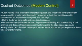
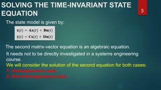
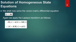
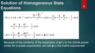
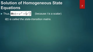
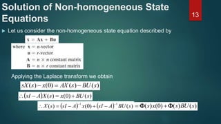
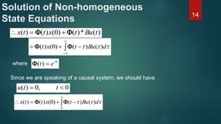
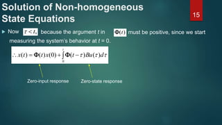
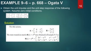
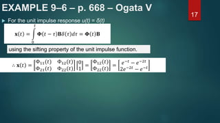
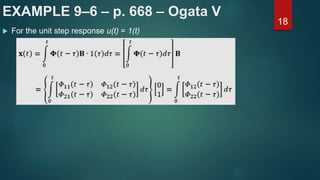
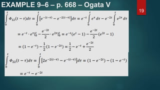
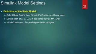
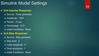
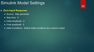
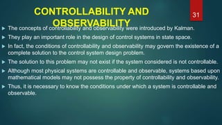
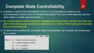
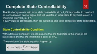
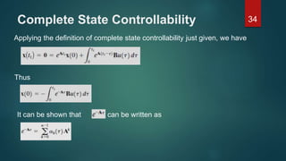
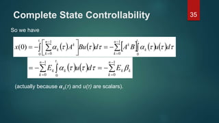
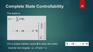
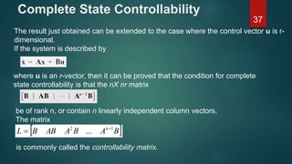
The document discusses concepts related to linear time-invariant systems represented by state-space models. It provides: 1) An overview of desired learning outcomes related to solving state equations and understanding controllability and observability. 2) Details on solving the homogeneous and non-homogeneous state equations, including definitions of zero-state and zero-input responses. 3) The condition for a system to be completely state controllable, which is that the controllability matrix must be of full rank.

1. Dynamic Systems and Control
Engineering
Spring Semester
1
Instructor: Prof. Amr Sharawi
TA: Eng. Amira Gaber
Eng. Asmaa Mohamed

2. Desired Outcomes (Modern Control) 2
Know how to solve the matrix differential equation of a linear time-invariant system
represented by a state variable model in response to the initial conditions and to
standard inputs, especially unit impulse and unit step.
Define the terms zero-state and zero-input response.
Understand and appreciate the role of system controllability and observability in the
analysis and design of feedback control systems using the state space approach.
Apply Matlab and Simulink to compute the zero-state and zero-input response of linear
time invariant systems.

3. SOLVING THE TIME-INVARIANT STATE
EQUATION 3
The state model is given by:
The second matrix-vector equation is an algebraic equation.
It needs not to be directly investigated in a systems engineering
course.
We will consider the solution of the second equation for both cases:
1. Homogeneous case
2. Non-homogeneous case

4. Solution of Homogeneous State
Equations
 Before we solve vector-matrix differential equations, let us review the
solution of the scalar differential equation:
4
To obtain the solution to that equation we apply the Laplace
transform as follows:

5. Solution of Homogeneous State
Equations
 We shall now solve the vector-matrix differential equation
5
Again we apply the Laplace transform as follows:

6. Solution of Homogeneous State
Equations 6
Because of the similarity of the expansion of 𝜙(t) to the infinite power
series for a scalar exponential, we call 𝜙(t) the matrix exponential

7. Solution of Homogeneous State
Equations
 Thus,
7
 tAAt
eet )(
𝜙(t) is called the state-transition matrix.
(because t is a scalar)

8. Properties of the State-Transition Matrix
8
)()( tAAee
dt
d
t AtAt
 

6.

9. Structure of the Matrix Exponential
9
 In general













tatata
tatata
tatata
At
nnnn
n
n
eee
eee
eee
e
...
............
...
...
21
22221
11211
(because the exponential function is
nonlinear, whereas the matrix is a linear
operator)
Special Case













ta
ta
ta
At
nn
e
e
e
e
...00
............
0...0
0...0
22
11
If and only if A is diagonal.

10. Special Case
10Proof:




























0
0
22
0
11
!
)(
...00
............
0...
!
)(
0
0...0
!
)(
k
k
nn
k
k
k
k
At
k
ta
k
ta
k
ta
e













ta
ta
ta
nn
e
e
e
...00
............
0...0
0...0
22
11
 
 
 
  














k
nn
k
k
k
ta
ta
ta
At
...00
............
0...0
0...0
22
11

11. EXAMPLE 9–5 – p. 665 – Ogata V
11
Solution
)(s
)(t







)()(
)()(
2221
1211
ss
ss



12. EXAMPLE 9–5 – p. 665 – Ogata V
12



















1
1
2
2
1
2
2
2
2
1
1
1
2
1
1
2
)(
ssss
sssss




















1
1
2
2
1
2
2
2
2
1
1
1
2
1
1
2
)(
ssss
sssss
)(t

13. Solution of Non-homogeneous State
Equations
 Let us consider the non-homogeneous state equation described by
13
Applying the Laplace transform we obtain
)()()0()( sBUsAXxssX 
  )()0()( sBUxsXAsI 
    )()0()(
11
sBUAsIxAsIsX

 )()()0()( sBUsxs  

14. Solution of Non-homogeneous
State Equations 14



  dButxt )()()0()( 
where At
et )(
Since we are speaking of a causal system, we should have
0,0)(  ttu



0
)()()0()()(  dButxttx 
)(*)()0()()( tButxttx  

15. Solution of Non-homogeneous
State Equations
 Now
15
,t because the argument t in )(t must be positive, since we start
measuring the system’s behavior at t = 0.
 
t
dButxttx
0
)()()0()()( 
Zero-input response Zero-state response

16. EXAMPLE 9–6 – p. 668 – Ogata V
 Obtain the unit impulse and the unit step response of the following
system. Assume zero initial conditions.
16
Solution

17. EXAMPLE 9–6 – p. 668 – Ogata V
17
 For the unit impulse response u(t) = δ(t)
𝐱 𝑡 =
0
𝑡
𝚽 𝑡 − 𝜏 𝐁𝛿 𝜏 𝑑𝜏 = 𝚽 𝑡 𝐁
using the sifting property of the unit impulse function.
∴ 𝐱 𝑡 =
Φ11(𝑡) Φ12(𝑡)
Φ21(𝑡) Φ22(𝑡)
0
1
=
Φ12(𝑡)
Φ22(𝑡)
= 𝑒−𝑡 − 𝑒−2𝑡
2𝑒−2𝑡 − 𝑒−𝑡

18. EXAMPLE 9–6 – p. 668 – Ogata V
18
 For the unit step response u(t) = 1(t)

19. EXAMPLE 9–6 – p. 668 – Ogata V
19

20. EXAMPLE 9–6 – p. 668 – Ogata V
20

21. MATLAB APPLICATIONS1
 Plotting and computing the zero-input response
 Plotting and computing the unit impulse response
 Plotting and computing the unit step response
21
1For all MATLAB examples in this course only the command lines (code statements)
are displayed. No results are furnished.

22. Defining the System and its State Model
22
u
x
x
x
x






























1
0
32
10
2
1
2
1
  






2
1
01
x
x
y












2
1
20
10
x
x
MATLAB Code

23. Zero-input Response 23

24. Unit Impulse Response 24

25. Unit Step Response 25

26. Simulink Applications
 Zero-input Response
 Unit Impulse Response
 Unit Step Rsponse
26

27. Simulink Models 27
Unit impulse response
Zero-input & Unit step response

28. Simulink Model Settings
 Definition of the State Model:
 Select State Space from Simulink’s Continuous library tools
 Define each of A, B, C, D in the same way as MATLAB.
 Initial Conditions: Depending on the input signal
28

29. Simulink Model Settings
 Unit Impulse Response:
 Source: Pulse generator
 Amplitude: 1000
 Period: 10 sec
 Percentage: 0.01
 Initial Conditions: None
 Unit Step Response:
 Source: Step generator
 Step time: 0
 Initial amplitude: 0
 Final amplitude: 1
 Initial Conditions: None
29

30. Simulink Model Settings
 Zero-input Response:
 Source: Step generator
 Step time: 0
 Initial amplitude: 0
 Final amplitude: 0
 Initial Conditions: Define initial conditions as a column vector
30

31. CONTROLLABILITY AND
OBSERVABILITY The concepts of controllability and observability were introduced by Kalman.
 They play an important role in the design of control systems in state space.
 In fact, the conditions of controllability and observability may govern the existence of a
complete solution to the control system design problem.
 The solution to this problem may not exist if the system considered is not controllable.
 Although most physical systems are controllable and observable, systems based upon
mathematical models may not possess the property of controllability and observability.
 Thus, it is necessary to know the conditions under which a system is controllable and
observable.
31

32. Complete State Controllability
 A system is said to be controllable at time to if it is possible by means of an
unconstrained control vector to transfer the system from any initial state x(to) to any
other state in a finite interval of time, t.
 By unconstrained control vector we understand an input vector u(t) that can draw any
path in the state space during its course from to to t, without there being any boundary
that may limit that path.
 To derive the condition for complete state controllability, we consider the continuous-
time system.
32

33. Complete State Controllability 33
That kind of system is said to be state controllable at t = to if it is possible to construct
an unconstrained control signal that will transfer an initial state to any final state in a
finite time interval to ≤ t ≤ t1.
If every state is controllable, then the system is said to be completely state controllable.
State Controllability Condition
Without loss of generality, we can assume that the final state is the origin of the
state space and that the initial time is zero, or to=0.
The solution of the state equation is given by:

34. Complete State Controllability 34
Applying the definition of complete state controllability just given, we have
Thus
It can be shown that can be written as

35. Complete State Controllability 35
So we have
           duBAdBuAx
t
k
n
k
k
t n
k
k
k  









11
0
1
00
1
0
)0(
    k
n
k
k
t
k
n
k
k EduE  





1
00
1
0
1
    k
n
k
k
t
k
n
k
k EduE  





1
00
1
0
1
(actually because 𝜶k(τ) and u(τ) are scalars).

36. Complete State Controllability 36
This leads to
For a unique solution vector β to exist, the matrix
must be non-singular, i.e., of rank = n.

37. Complete State Controllability
37
The result just obtained can be extended to the case where the control vector u is r-
dimensional.
If the system is described by
where u is an r-vector, then it can be proved that the condition for complete
state controllability is that the nХ nr matrix
be of rank n, or contain n linearly independent column vectors.
The matrix
 BABAABBL n 12
... 

is commonly called the controllability matrix.

38. EXAMPLE 9–10 – p. 677 – Ogata V
38
Consider the system given by
Solution

39. EXAMPLE 9–11 – p. 678 – Ogata V
39
Consider the system given by
Solution

40. Complete State Controllability in the s-
plane
 The condition for complete state controllability can be stated in terms of transfer
functions or transfer matrices.
 It can be proved that a necessary and sufficient condition for complete state
controllability is that no pole-zero cancellation occur in the transfer function or transfer
matrix.
 If cancellation occurs, the system cannot be controlled in the direction of the canceled
mode.
40

41. EXAMPLE 9–13 – p. 680 – Ogata V
41
Consider the following transfer function:
Solution
Clearly, cancellation of the factor (s+2.5) occurs in the numerator and
denominator of this transfer function. (Thus one degree of freedom is lost.)
Because of this cancellation, this system is not completely state controllable.

42. Output Controllability
 In the practical design of a control system, we may want to control the output rather
than the state of the system.
 Complete state controllability is neither necessary nor sufficient for controlling the
output of the system.
 For this reason, it is desirable to define separately complete output controllability.
42

43. Output Controllability 43
Consider the system described by

44. Output Controllability
 The above system is said to be completely output controllable if it is possible to
construct an unconstrained control vector u(t) that will transfer any given initial output
y(to) to any final output y(t1) in a finite time interval to ≤ t ≤ t1.
 It can be proved that the same system is completely output controllable if and only if
the mХ(n+1)r matrix
44
 DBCABCACABCBP n 12
... 

is of rank m.

45. Uncontrollable System
 An uncontrollable system has a subsystem that is physically
disconnected from the input.
45

46. Stabilizability
 For a partially controllable system, if the uncontrollable modes are stable and the
unstable modes are controllable, the system is said to be stabilizable.
 For example, the system defined by
46
is not state controllable.
The stable mode that corresponds to the eigenvalue of –1 is not controllable.
The unstable mode that corresponds to the eigenvalue of 1 is controllable.
Such a system can be made stable by the use of a suitable feedback.
Thus this system is stabilizable.