State space represenation

1. • Objectives:
Introduction
Differential Equations
Applications to Circuits
Solutions to the State Equations
•
STATE SPACE REPRESENTATION
THE STATE EQUATIONS

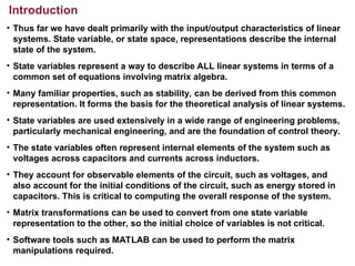
2. • Thus far we have dealt primarily with the input/output characteristics of linear
systems. State variable, or state space, representations describe the internal
state of the system.
• State variables represent a way to describe ALL linear systems in terms of a
common set of equations involving matrix algebra.
• Many familiar properties, such as stability, can be derived from this common
representation. It forms the basis for the theoretical analysis of linear systems.
• State variables are used extensively in a wide range of engineering problems,
particularly mechanical engineering, and are the foundation of control theory.
• The state variables often represent internal elements of the system such as
voltages across capacitors and currents across inductors.
• They account for observable elements of the circuit, such as voltages, and
also account for the initial conditions of the circuit, such as energy stored in
capacitors. This is critical to computing the overall response of the system.
• Matrix transformations can be used to convert from one state variable
representation to the other, so the initial choice of variables is not critical.
• Software tools such as MATLAB can be used to perform the matrix
manipulations required.
Introduction

3. State Equations
• Let us define the state of the system by an N-element column vector, x(t):
Note that in this development, v(t) will be the input, y(t) will be the output, and
x(t) is used for the state variables.
• Any system can be modeled by the following state equations:
• This system model can handle
single input/single output systems,
or multiple inputs and outputs.
• The equations above can be
implemented using the signal flow
graph shown to the right.
• Works for ALL linear systems!
 t
N
N
t
x
t
x
t
x
t
x
t
x
t
x
t )
(
)
(
)
(
)
(
)
(
)
(
)
( 2
1
2
1
















x
outputs
of
number
:
:
:
1
:
)
(
)
(
)
(
inputs
of
number
:
:
:
1
:
)
(
)
(
)
(
q
qxp
qxN
qx
t
t
x
t
p
Nxp
NxN
Nx
t
t
t
D
C
y
Dv
C
y
B
A
x
Bv
Ax
x






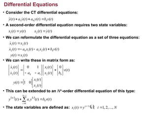
4. • Consider the CT differential equations:
• A second-order differential equation requires two state variables:
• We can reformulate the differential equation as a set of three equations:
• We can write these in matrix form as:
• This can be extended to an Nth
-order differential equation of this type:
• The state variables are defined as:
Differential Equations
)
(
)
(
)
(
)
( 0
0
1 t
v
b
t
y
a
t
y
a
t
y 

 


)
(
)
(
)
(
)
( 2
1 t
y
t
x
t
y
t
x 


)
(
)
(
)
(
)
(
)
(
)
(
)
(
)
(
1
0
2
1
1
0
2
2
1
t
x
t
y
t
v
b
t
x
a
t
x
a
t
x
t
x
t
x








  


































)
(
)
(
0
1
)
(
)
(
0
)
(
)
(
1
0
)
(
)
(
2
1
0
2
1
1
0
2
1
t
x
t
x
t
y
t
v
b
t
x
t
x
a
a
t
x
t
x


   
)
(
)
(
)
( 0
1
0
t
v
b
t
y
a
t
y
N
i
i
i
N




  N
i
t
y
t
x i
i ...,
,
2
,
1
,
)
( )
1
(

 

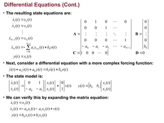
5. • The resulting state equations are:
• Next, consider a differential equation with a more complex forcing function:
• The state model is:
• We can verify this by expanding the matrix equation:
Differential Equations (Cont.)
)
(
)
(
)
(
)
(
)
(
)
(
)
(
)
(
)
(
)
(
)
(
1
0
1
0
1
1
3
2
2
1
t
x
t
y
t
v
b
t
x
a
t
x
t
x
t
x
t
x
t
x
t
x
t
x
N
i
i
i
N
N
N

















  0
0
0
0
1
0
0
0
1
0
0
0
1
0
0
0
0
1
0
0
1
2
1
0









































D
C
B
A











b
a
a
a
a N
)
(
)
(
)
(
)
(
)
( 0
1
0
1 t
v
b
t
v
b
t
y
a
t
y
a
t
y 


 



  


































)
(
)
(
)
(
)
(
1
0
)
(
)
(
1
0
)
(
)
(
2
1
1
0
2
1
1
0
2
1
t
x
t
x
b
b
t
y
t
v
t
x
t
x
a
a
t
x
t
x


)
(
)
(
)
(
)
(
)
(
)
(
)
(
)
(
)
(
2
1
1
0
2
1
1
0
2
2
1
t
x
b
t
x
b
t
y
t
v
t
x
a
t
x
a
t
x
t
x
t
x










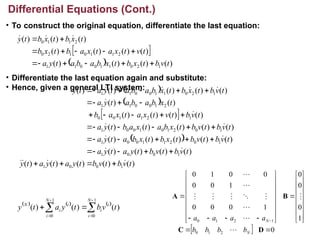
6. • To construct the original equation, differentiate the last equation:
• Differentiate the last equation again and substitute:
• Hence, given a general LTI system:
Differential Equations (Cont.)
 
  )
(
)
(
)
(
)
(
)
(
)
(
)
(
)
(
)
(
)
(
)
(
1
2
0
1
1
0
0
1
1
2
1
1
0
1
2
0
2
1
1
0
t
v
b
t
x
b
t
x
b
a
b
a
t
y
a
t
v
t
x
a
t
x
a
b
t
x
b
t
x
b
t
x
b
t
y












 


 
 
 
 
)
(
)
(
)
(
)
(
)
(
)
(
)
(
)
(
)
(
)
(
)
(
)
(
)
(
)
(
)
(
)
(
)
(
)
(
)
(
)
(
)
(
)
(
)
(
)
(
)
(
)
(
)
(
)
(
)
(
)
(
1
0
0
1
1
0
0
1
1
0
2
1
1
0
0
1
1
0
2
1
0
1
0
0
1
1
2
1
1
0
0
2
1
0
0
1
1
1
2
0
1
1
0
0
1
1
t
v
b
t
v
b
t
y
a
t
y
a
t
y
t
v
b
t
v
b
t
y
a
t
y
a
t
v
b
t
v
b
t
x
b
t
x
b
a
t
y
a
t
v
b
t
v
b
t
x
b
a
t
x
a
b
t
y
a
t
v
b
t
v
t
x
a
t
x
a
b
t
x
b
a
b
a
t
y
a
t
v
b
t
x
b
t
x
b
a
b
a
t
y
a
t
y






















































     








1
0
1
0
)
(
)
(
)
(
N
i
i
i
N
i
i
i
N
t
v
b
t
y
a
t
y
  0
1
0
0
0
1
0
0
0
1
0
0
0
0
1
0
2
1
0
1
2
1
0









































D
C
B
A
N
N
b
b
b
b
a
a
a
a












7. Application to Circuits (Using Slide #3)
)
(
1
)
(
1
)
(
t
v
RC
t
y
RC
dt
t
dy

 )
(
1
)
(
1
)
(
)
(
2
2
t
v
LC
t
y
LC
dt
t
dy
L
R
dt
t
y
d









 
    0
1
1
1
0
0




















D
C
B
A
RC
b
RC
a
  





































)
(
1
)
(
)
(
1
)
(
1
)
(
1
1
1
t
x
t
y
t
v
RC
t
x
RC
t
x
   0
0
1
/
1
0
0
/
/
1
1
0
1
0
0
1
0


































D
C
B
A
LC
b
L
R
LC
a
a
  


































)
(
)
(
0
1
)
(
)
(
/
1
0
)
(
)
(
/
/
1
1
0
)
(
)
(
2
1
2
1
2
1
t
x
t
x
t
y
t
v
LC
t
x
t
x
L
R
LC
t
x
t
x



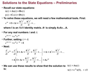
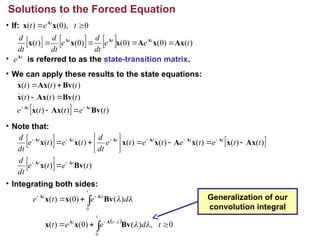
8. • Recall our state equations:
• To solve these equations, we will need a few mathematical tools. First:
where I is an NxN identity matrix. Ak
is simply AxAx…A.
• For any real numbers t and :
• Further, setting  = -t:
• Next:
• We can use these results to show that the solution to
is:
Solutions to the State Equations – Preliminaries
)
(
)
(
)
(
)
(
)
(
)
(
t
t
x
t
t
t
t
Dv
C
y
Bv
Ax
x











!
3
!
2
3
3
2
2
t
t
t
e t A
A
A
I
A

 A
A
A
e
e
e t
t

 )
(
I
A
A
A

 
 t
t
t
e
e
e )
( 
t
t
e
t
t
t
t
t
t
t
t
dt
d
e
dt
d
A
A
A
A
A
A
I
A
A
A
A
A
A
A
I
































!
3
!
2
!
2
!
3
!
2
3
3
2
2
2
3
2
3
3
2
2
)
(
)
( t
t Ax
x 

0
),
0
(
)
( 
 t
e
t t
x
x A

9. • If:
• is referred to as the state-transition matrix.
• We can apply these results to the state equations:
• Note that:
• Integrating both sides:
Solutions to the Forced Equation
t
eA
      )
(
)
0
(
)
0
(
)
0
(
)
( t
e
e
dt
d
e
dt
d
t
dt
d t
t
t
Ax
x
A
x
x
x A
A
A




0
),
0
(
)
( 
 t
e
t t
x
x A
  )
(
)
(
)
(
)
(
)
(
)
(
)
(
)
(
)
(
t
e
t
t
e
t
t
t
t
t
t
t
t
Bv
Ax
x
Bv
Ax
x
Bv
Ax
x
A
A 










   
  )
(
)
(
)
(
)
(
)
(
)
(
)
(
)
(
)
(
t
e
t
e
dt
d
t
t
e
t
e
t
e
t
e
dt
d
t
e
t
e
dt
d
t
t
t
t
t
t
t
t
Bv
x
Ax
x
x
A
x
x
x
x
A
A
A
A
A
A
A
A




















 


 
0
,
)
(
)
0
(
)
(
)
(
)
0
(
)
(
0
0











t
d
e
e
t
d
e
t
e
t
t
t
t
t






Bv
x
x
Bv
x
x
A
A
A
A Generalization of our
convolution integral

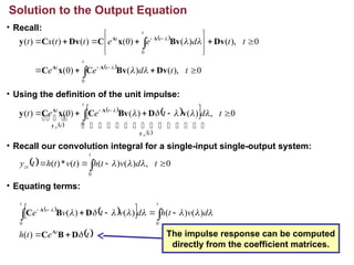
10. • Recall:
• Using the definition of the unit impulse:
• Recall our convolution integral for a single-input single-output system:
• Equating terms:
Solution to the Output Equation
 
 
0
),
(
)
(
)
0
(
0
),
(
)
(
)
0
(
)
(
)
(
)
(
0
0






















t
t
d
e
e
t
t
d
e
e
t
t
x
t
t
t
t
t
t
t
Dv
Bv
C
x
C
Dv
Bv
x
C
Dv
C
y
A
A
A
A






 
 
 
 
 
0
,
)
(
)
(
)
0
(
)
(
0




 


t
d
t
e
e
t
t
t
t
t
t
zs
zi 




 





 


 

y
A
y
A
v
D
Bv
C
x
C
y 





 
 
 
 
t
e
t
h
d
v
t
h
d
v
t
v
e
t
t t
t










D
B
C
D
B
C
A
A






 


)
(
)
(
)
(
)
(
)
(
0 0
  0
,
)
(
)
(
)
(
*
)
(
0



  t
d
v
t
h
t
v
t
h
t
y
t
zs 


The impulse response can be computed
directly from the coefficient matrices.

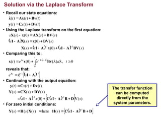
11. Solution via the Laplace Transform
• Recall our state equations:
• Using the Laplace transform on the first equation:
• Comparing this to:
reveals that:
• Continuing with the output equation:
• For zero initial conditions:
)
(
)
(
)
(
)
(
)
(
)
(
t
t
x
t
t
t
t
Dv
C
y
Bv
Ax
x





 
    )
(
)
0
(
)
(
)
(
)
0
(
)
(
)
(
)
(
)
0
(
)
(
1
1
s
s
s
s
s
s
s
s
s
s
s
BV
A
I
x
A
I
X
BV
x
X
A
I
BV
AX
x
X












 
0
,
)
(
)
0
(
)
(
0


 


t
d
e
e
t
t
t
t



Bv
x
x A
A
 
 
1
1 


 A
I
A
s
e t
L
   
  )
(
)
0
(
)
(
)
(
)
(
)
(
)
(
)
(
1
1
s
s
x
s
s
s
s
t
t
x
t
V
D
B
A
I
C
A
I
DV
CX
Y
Dv
C
y











 
 
D
B
A
I
C
H
X
H
Y 



 1
)
(
where
)
(
)
(
)
( s
s
s
s
s
The transfer function
can be computed
directly from the
system parameters.

12. Summary
• Introduced the concept of a state variable.
• Described a linear system in terms of the general state equation.
• Demonstrated a process for deriving the state equations from a differential
equation with a simple forcing function.
• Generalized this to an Nth-order differential equation with a more complex
forcing function.
• Demonstrated these techniques on a 1st
-order (RC) and 2nd
-order (RLC) circuit.
• Observation: We have now encapsulated all passive circuit analysis (RLCs)
into a single matrix equation. In fact, we now have a unified representation for
all linear time-invariant systems.
• Introduced the time-domain and Laplace transform-based solutions to the
state equations.
• Even nonlinear (and non-time-invariant) systems can be modeled using these
techniques. However, the resulting differential equations are more complex.
Fortunately, we have powerful numerical modeling techniques to handle such
problems.