asdasd

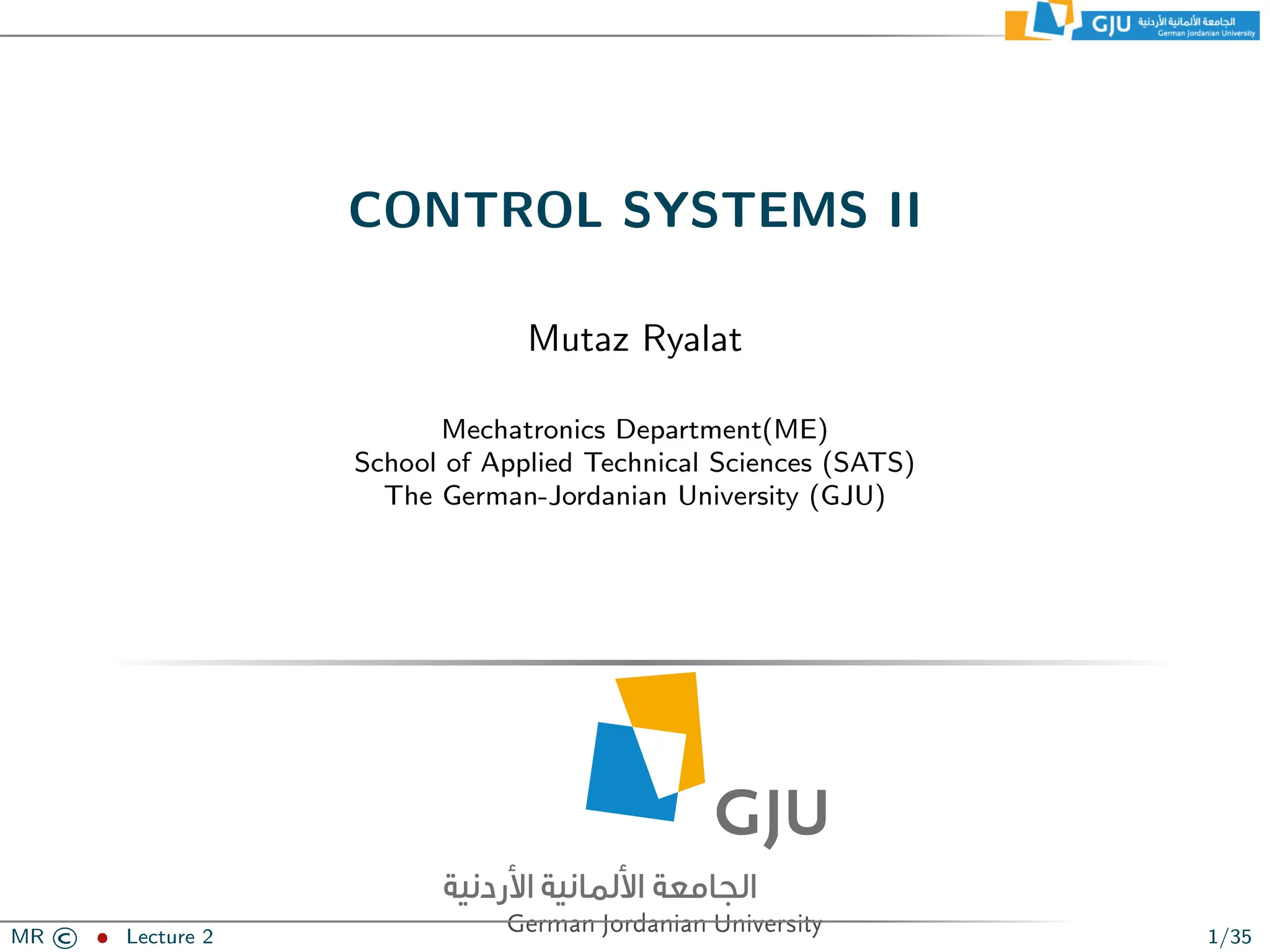
1. CONTROL SYSTEMS II
Mutaz Ryalat
Mechatronics Department(ME)
School of Applied Technical Sciences (SATS)
The German-Jordanian University (GJU)
MR © ˆ Lecture 2 1/35

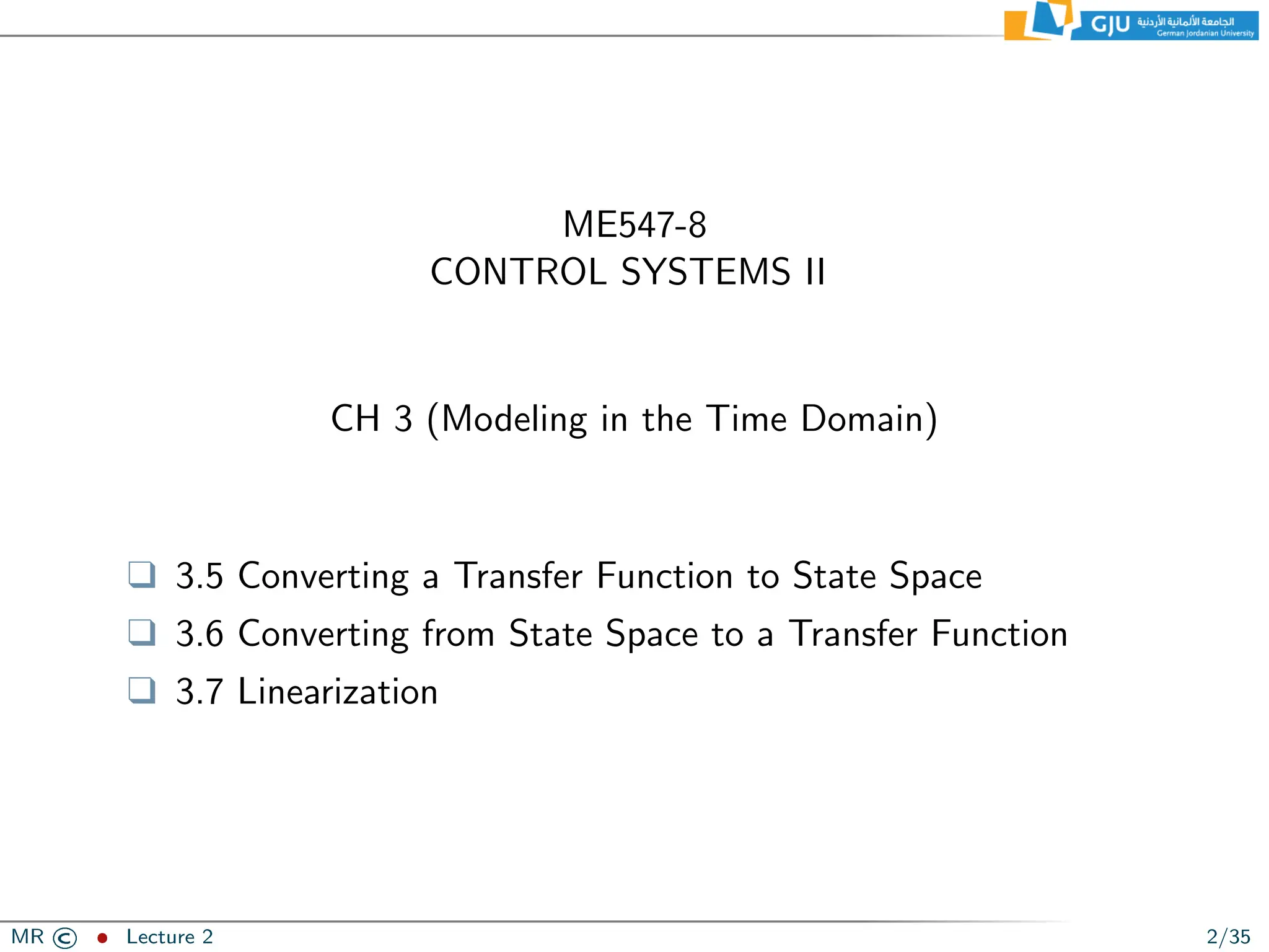
2. ME547-8
CONTROL SYSTEMS II
CH 3 (Modeling in the Time Domain)
❑ 3.5 Converting a Transfer Function to State Space
❑ 3.6 Converting from State Space to a Transfer Function
❑ 3.7 Linearization
MR © ˆ Lecture 2 2/35

3. 3.5 Converting a Transfer Function to State Space
MR © ˆ Lecture 2 3/35

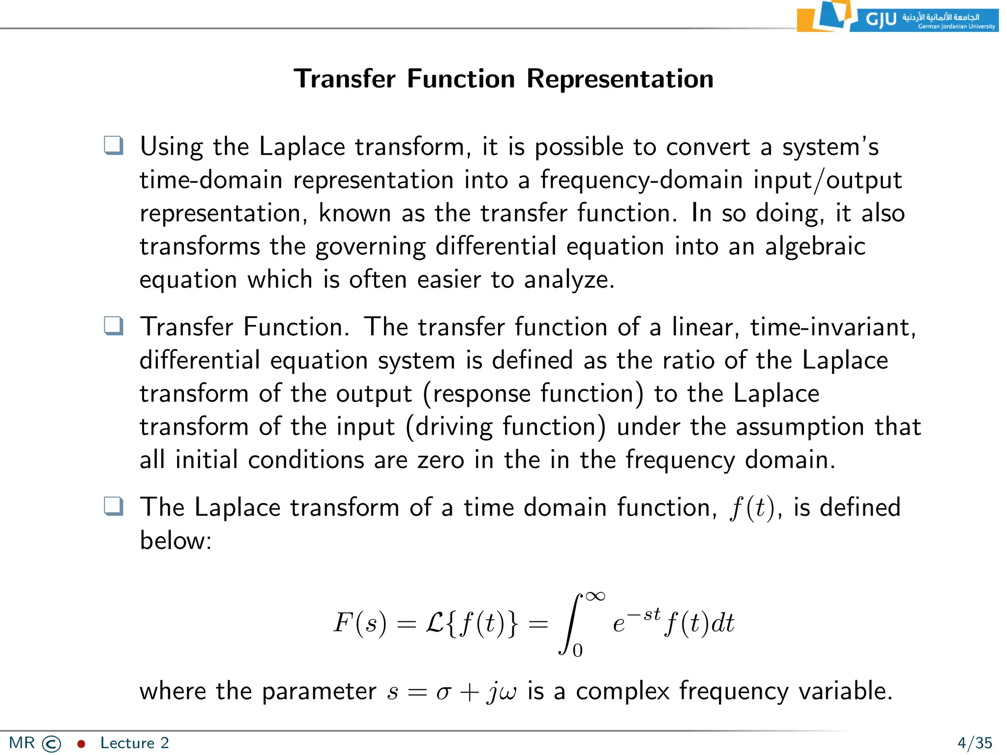
4. Transfer Function Representation
❑ Using the Laplace transform, it is possible to convert a system’s
time-domain representation into a frequency-domain input/output
representation, known as the transfer function. In so doing, it also
transforms the governing differential equation into an algebraic
equation which is often easier to analyze.
❑ Transfer Function. The transfer function of a linear, time-invariant,
differential equation system is defined as the ratio of the Laplace
transform of the output (response function) to the Laplace
transform of the input (driving function) under the assumption that
all initial conditions are zero in the in the frequency domain.
❑ The Laplace transform of a time domain function, f(t), is defined
below:
F(s) = L{f(t)} =
Z ∞
0
e−st
f(t)dt
where the parameter s = σ + jω is a complex frequency variable.
MR © ˆ Lecture 2 4/35

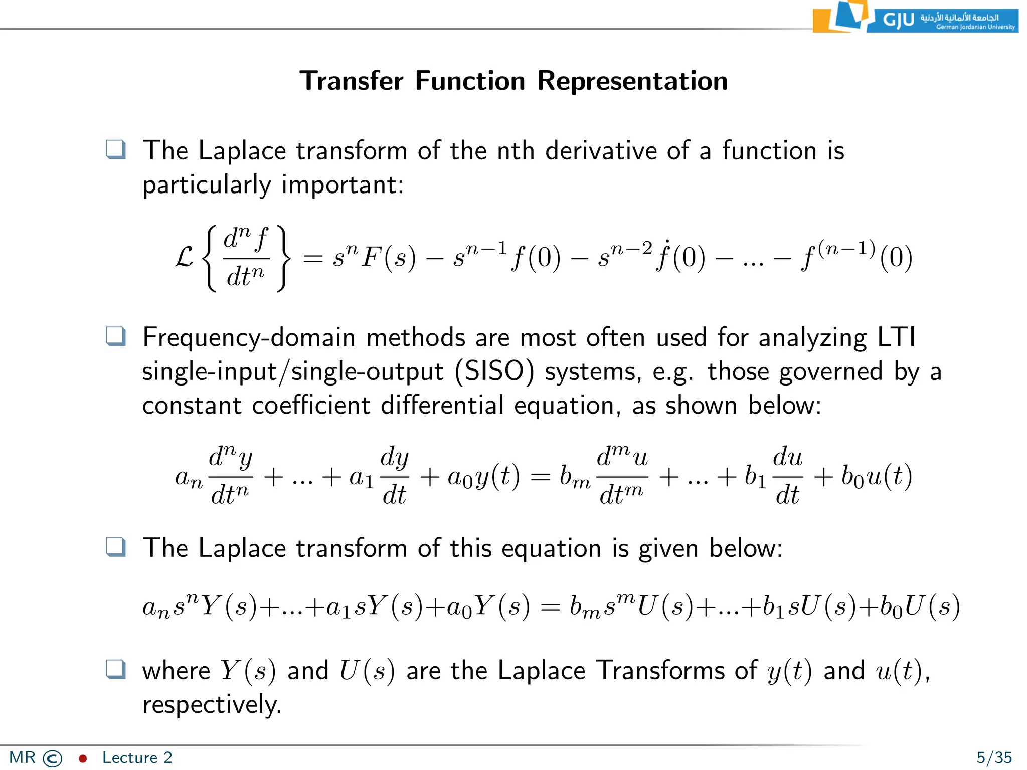
5. Transfer Function Representation
❑ The Laplace transform of the nth derivative of a function is
particularly important:
L
dn
f
dtn
= sn
F(s) − sn−1
f(0) − sn−2 ˙
f(0) − ... − f(n−1)
(0)
❑ Frequency-domain methods are most often used for analyzing LTI
single-input/single-output (SISO) systems, e.g. those governed by a
constant coefficient differential equation, as shown below:
an
dn
y
dtn
+ ... + a1
dy
dt
+ a0y(t) = bm
dm
u
dtm
+ ... + b1
du
dt
+ b0u(t)
❑ The Laplace transform of this equation is given below:
ansn
Y (s)+...+a1sY (s)+a0Y (s) = bmsm
U(s)+...+b1sU(s)+b0U(s)
❑ where Y (s) and U(s) are the Laplace Transforms of y(t) and u(t),
respectively.
MR © ˆ Lecture 2 5/35

6. Transfer Function Representation
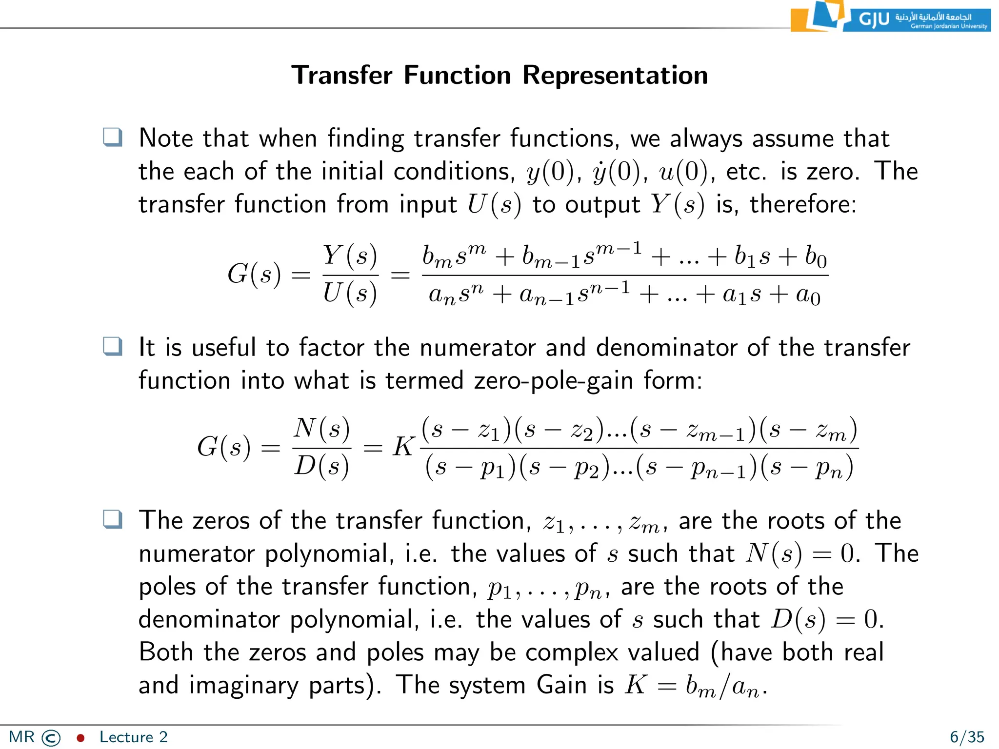
❑ Note that when finding transfer functions, we always assume that
the each of the initial conditions, y(0), ẏ(0), u(0), etc. is zero. The
transfer function from input U(s) to output Y (s) is, therefore:
G(s) =
Y (s)
U(s)
=
bmsm
+ bm−1sm−1
+ ... + b1s + b0
ansn + an−1sn−1 + ... + a1s + a0
❑ It is useful to factor the numerator and denominator of the transfer
function into what is termed zero-pole-gain form:
G(s) =
N(s)
D(s)
= K
(s − z1)(s − z2)...(s − zm−1)(s − zm)
(s − p1)(s − p2)...(s − pn−1)(s − pn)
❑ The zeros of the transfer function, z1, . . . , zm, are the roots of the
numerator polynomial, i.e. the values of s such that N(s) = 0. The
poles of the transfer function, p1, . . . , pn, are the roots of the
denominator polynomial, i.e. the values of s such that D(s) = 0.
Both the zeros and poles may be complex valued (have both real
and imaginary parts). The system Gain is K = bm/an.
MR © ˆ Lecture 2 6/35

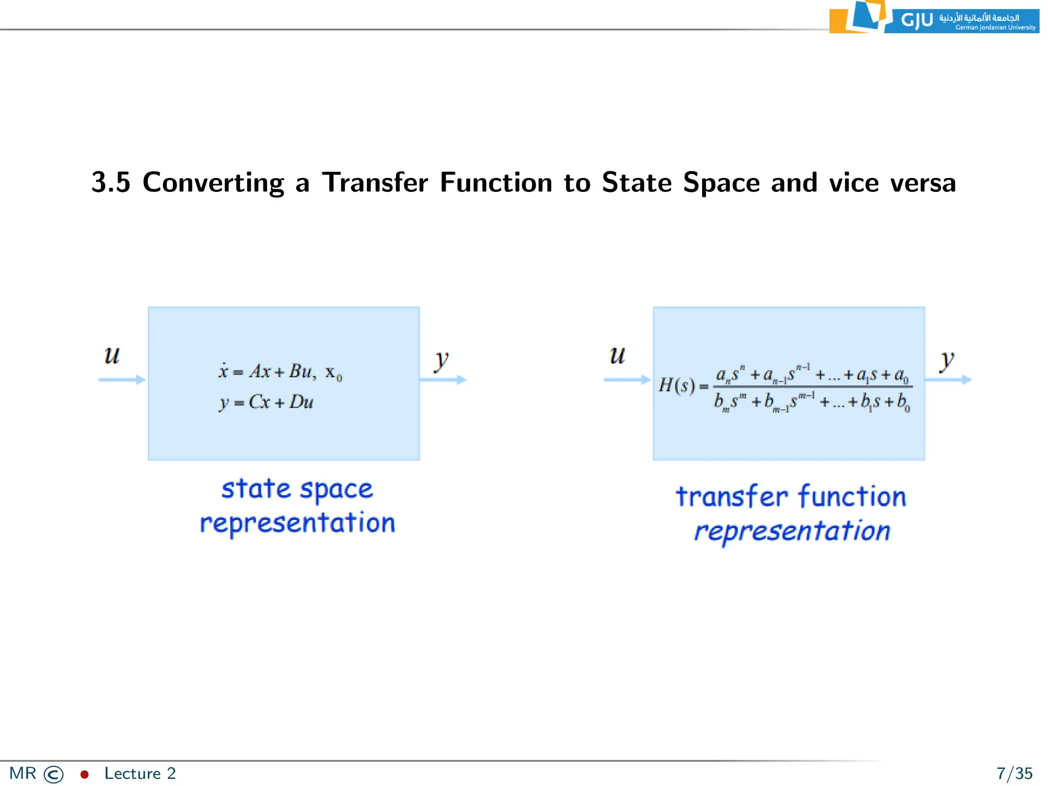
7. 3.5 Converting a Transfer Function to State Space and vice versa
MR © ˆ Lecture 2 7/35

8. TF’s to State-Space Models
❑ The goal is to develop a state-space model given a transfer function
for a system G(s).
❑ But there are three primary cases to consider:
❑ Simple numerator
G(s) =
Y (s)
U(s)
=
1
ansn + an−1sn−1 + ... + a1s + a0
❑ Numerator order less than denominator order
G(s) =
Y (s)
U(s)
=
bmsm
+ bm−1sm−1
+ ... + b1s + b0
ansn + an−1sn−1 + ... + a1s + a0
, m n
❑ Numerator equal to denominator order
G(s) =
Y (s)
U(s)
=
bmsm
+ bm−1sm−1
+ ... + b1s + b0
ansn + an−1sn−1 + ... + a1s + a0
, m = n
MR © ˆ Lecture 2 8/35

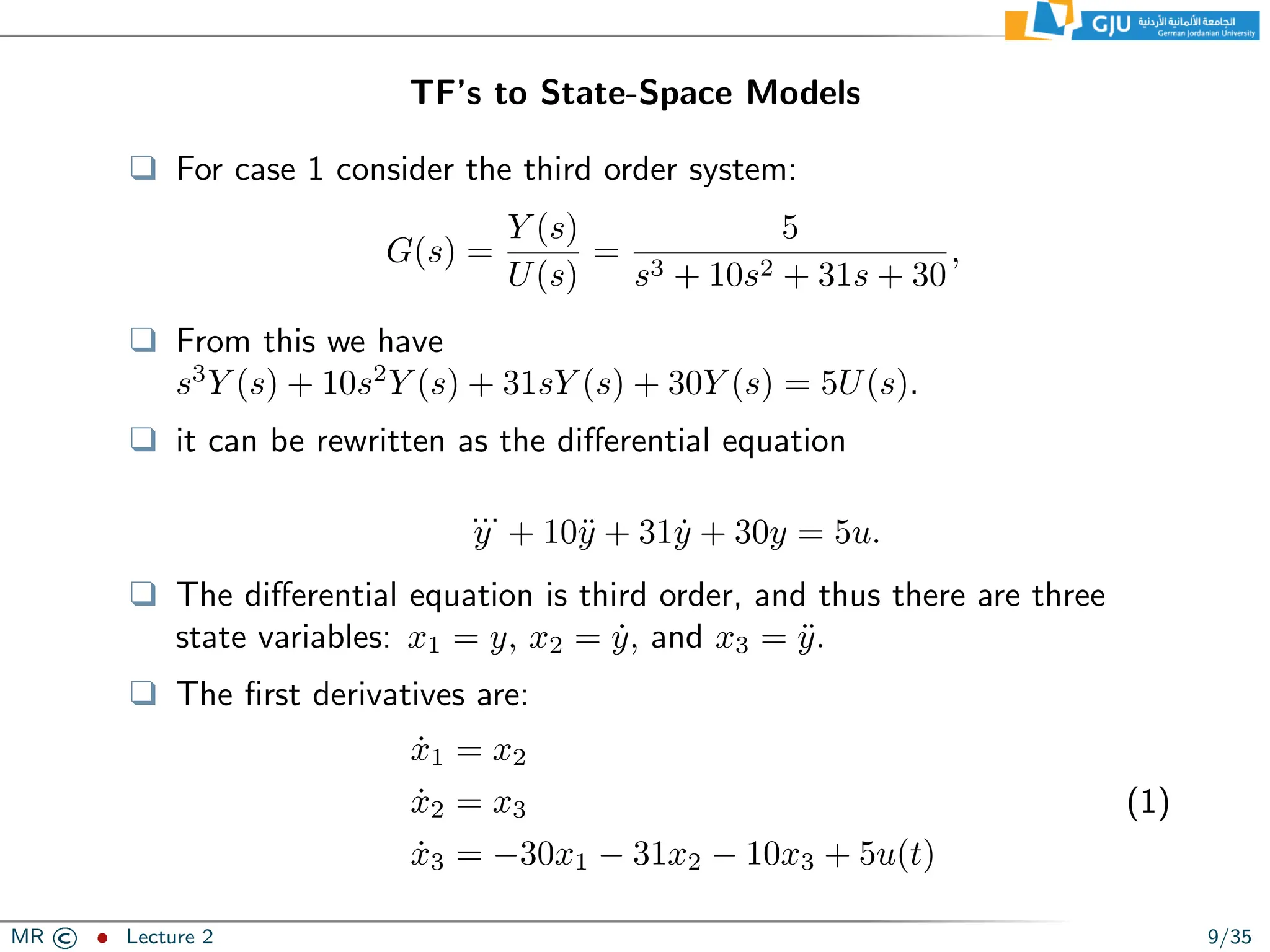
9. TF’s to State-Space Models
❑ For case 1 consider the third order system:
G(s) =
Y (s)
U(s)
=
5
s3 + 10s2 + 31s + 30
,
❑ From this we have
s3
Y (s) + 10s2
Y (s) + 31sY (s) + 30Y (s) = 5U(s).
❑ it can be rewritten as the differential equation
...
y + 10ÿ + 31ẏ + 30y = 5u.
❑ The differential equation is third order, and thus there are three
state variables: x1 = y, x2 = ẏ, and x3 = ÿ.
❑ The first derivatives are:
ẋ1 = x2
ẋ2 = x3
ẋ3 = −30x1 − 31x2 − 10x3 + 5u(t)
(1)
MR © ˆ Lecture 2 9/35

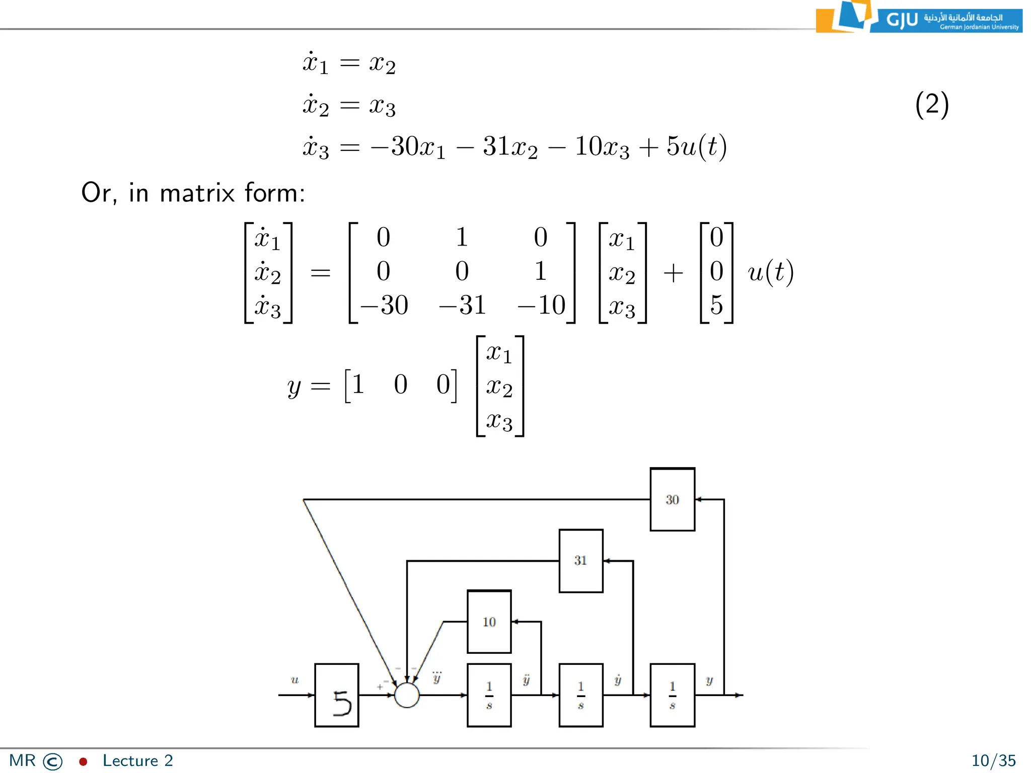
10. ẋ1 = x2
ẋ2 = x3
ẋ3 = −30x1 − 31x2 − 10x3 + 5u(t)
(2)
Or, in matrix form:


ẋ1
ẋ2
ẋ3

 =


0 1 0
0 0 1
−30 −31 −10




x1
x2
x3

 +


0
0
5

 u(t)
y =
1 0 0


x1
x2
x3


MR © ˆ Lecture 2 10/35

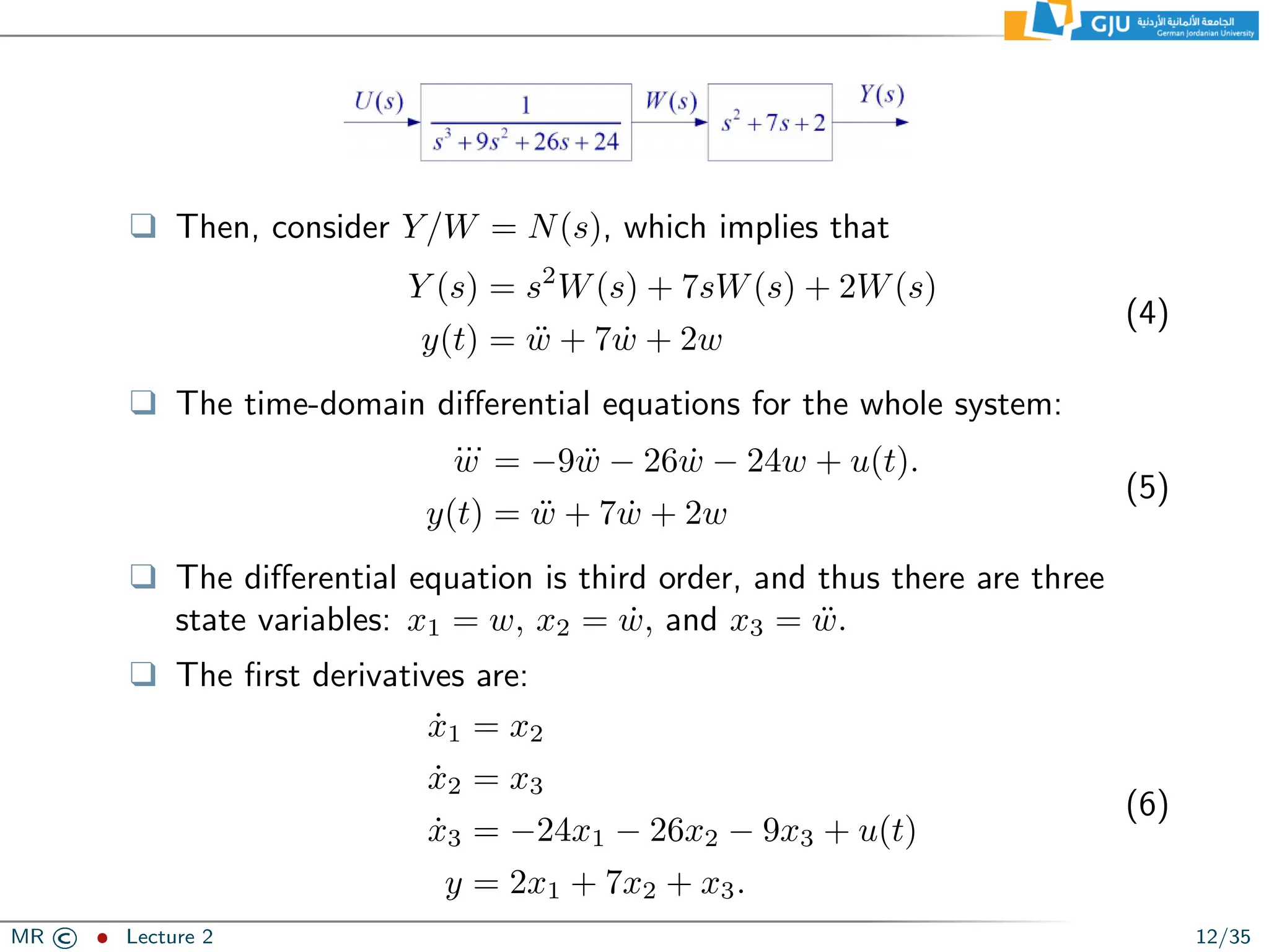
11. TF’s to State-Space Models
❑ For case 2 consider the third order system:
G(s) =
Y (s)
U(s)
=
s2
+ 7s + 2
s3 + 9s2 + 26s + 24
=
N(s)
D(s)
,
❑ Let
Y (s)
U(s)
=
Y (s)
W(s)
·
W(s)
U(s)
❑ where Y/W = N(s) and W/U = 1/D(s).
❑ The transfer function in block diagram cascade form
❑ Then representation of W/U = 1/D(s) is the same as case 1
s3
W(s) = −9s2
W(s) − 26sW(s) − 24W(s) + U(s)
...
w = −9ẅ − 26ẇ − 24w + u(t).
(3)
MR © ˆ Lecture 2 11/35

12. ❑ Then, consider Y/W = N(s), which implies that
Y (s) = s2
W(s) + 7sW(s) + 2W(s)
y(t) = ẅ + 7ẇ + 2w
(4)
❑ The time-domain differential equations for the whole system:
...
w = −9ẅ − 26ẇ − 24w + u(t).
y(t) = ẅ + 7ẇ + 2w
(5)
❑ The differential equation is third order, and thus there are three
state variables: x1 = w, x2 = ẇ, and x3 = ẅ.
❑ The first derivatives are:
ẋ1 = x2
ẋ2 = x3
ẋ3 = −24x1 − 26x2 − 9x3 + u(t)
y = 2x1 + 7x2 + x3.
(6)
MR © ˆ Lecture 2 12/35

13. ẋ1 = x2
ẋ2 = x3
ẋ3 = −24x1 − 26x2 − 9x3 + u(t)
y = 2x1 + 7x2 + x3.
(7)
Or, in matrix form:


ẋ1
ẋ2
ẋ3

 =


0 1 0
0 0 1
−24 −26 −9




x1
x2
x3

 +


0
0
1

 u(t)
y =
2 7 1


x1
x2
x3


MR © ˆ Lecture 2 13/35

14. 3.6 Converting from State Space to a Transfer Function
MR © ˆ Lecture 2 14/35

15. State space equations:
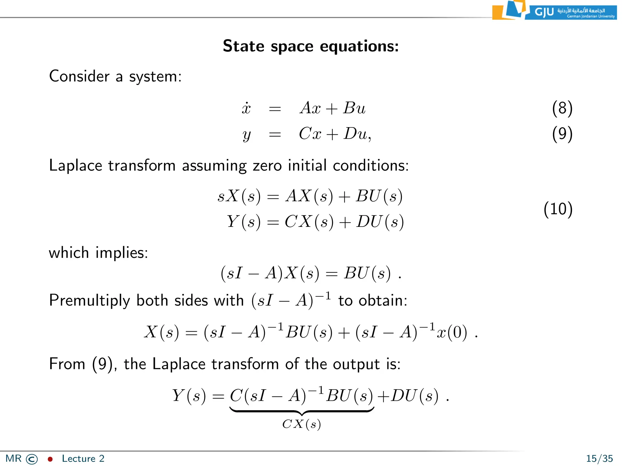
Consider a system:
ẋ = Ax + Bu (8)
y = Cx + Du, (9)
Laplace transform assuming zero initial conditions:
sX(s) = AX(s) + BU(s)
Y (s) = CX(s) + DU(s)
(10)
which implies:
(sI − A)X(s) = BU(s) .
Premultiply both sides with (sI − A)−1
to obtain:
X(s) = (sI − A)−1
BU(s) + (sI − A)−1
x(0) .
From (9), the Laplace transform of the output is:
Y (s) = C(sI − A)−1
BU(s)
| {z }
CX(s)
+DU(s) .
MR © ˆ Lecture 2 15/35

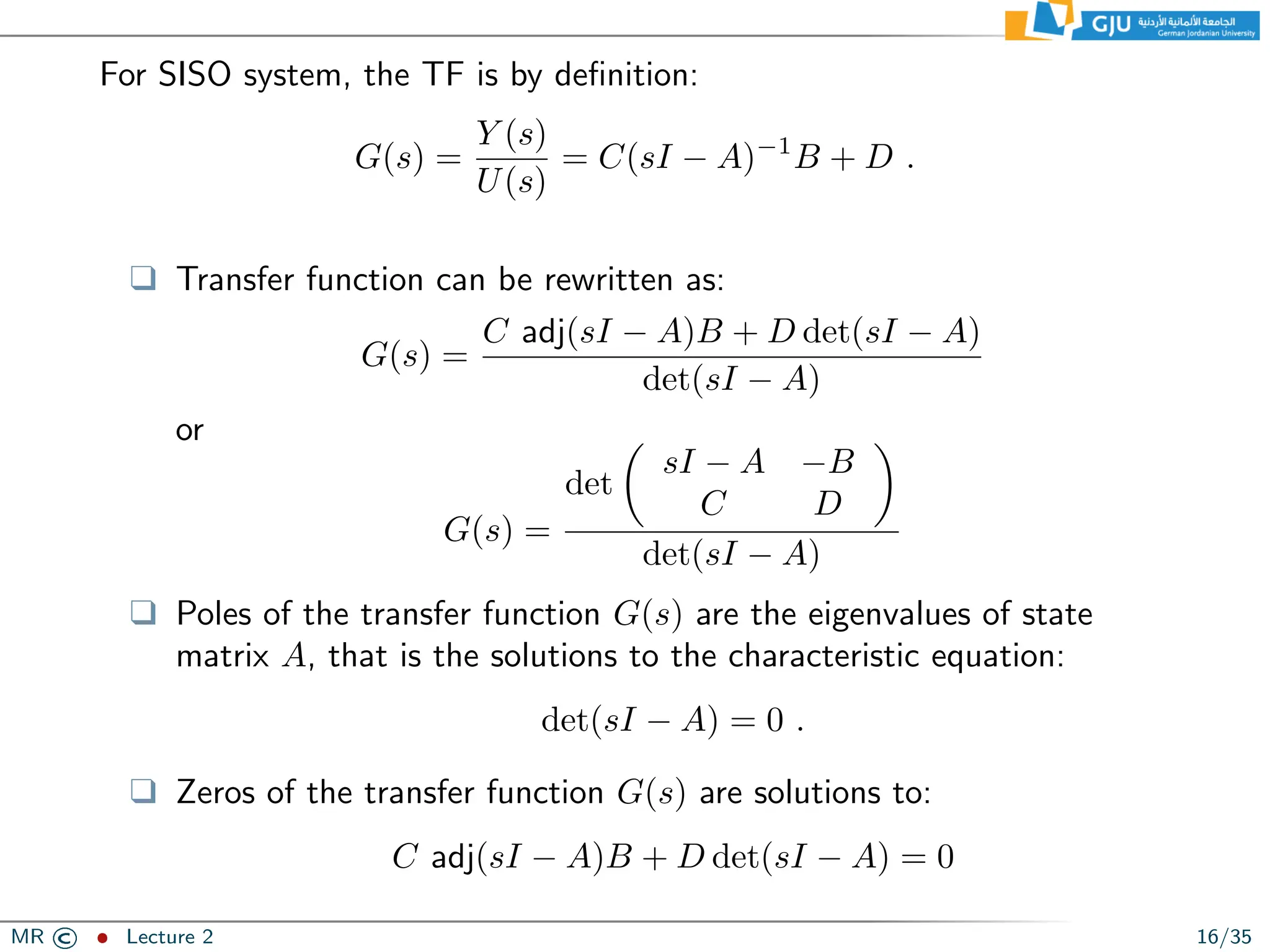
16. For SISO system, the TF is by definition:
G(s) =
Y (s)
U(s)
= C(sI − A)−1
B + D .
❑ Transfer function can be rewritten as:
G(s) =
C adj(sI − A)B + D det(sI − A)
det(sI − A)
or
G(s) =
det
sI − A −B
C D
det(sI − A)
❑ Poles of the transfer function G(s) are the eigenvalues of state
matrix A, that is the solutions to the characteristic equation:
det(sI − A) = 0 .
❑ Zeros of the transfer function G(s) are solutions to:
C adj(sI − A)B + D det(sI − A) = 0
MR © ˆ Lecture 2 16/35

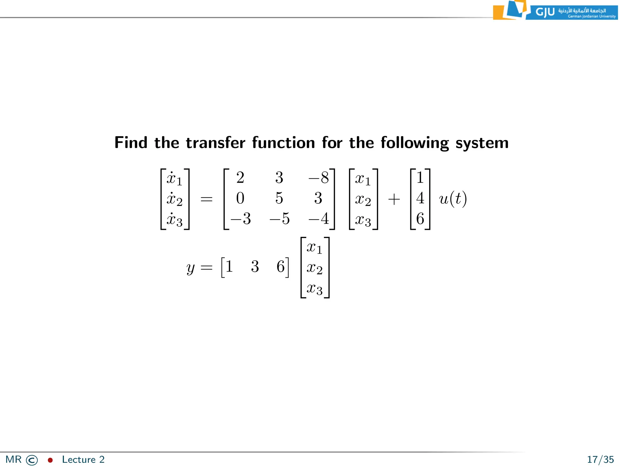
17. Find the transfer function for the following system


ẋ1
ẋ2
ẋ3

 =


2 3 −8
0 5 3
−3 −5 −4




x1
x2
x3

 +


1
4
6

 u(t)
y =
1 3 6


x1
x2
x3


MR © ˆ Lecture 2 17/35

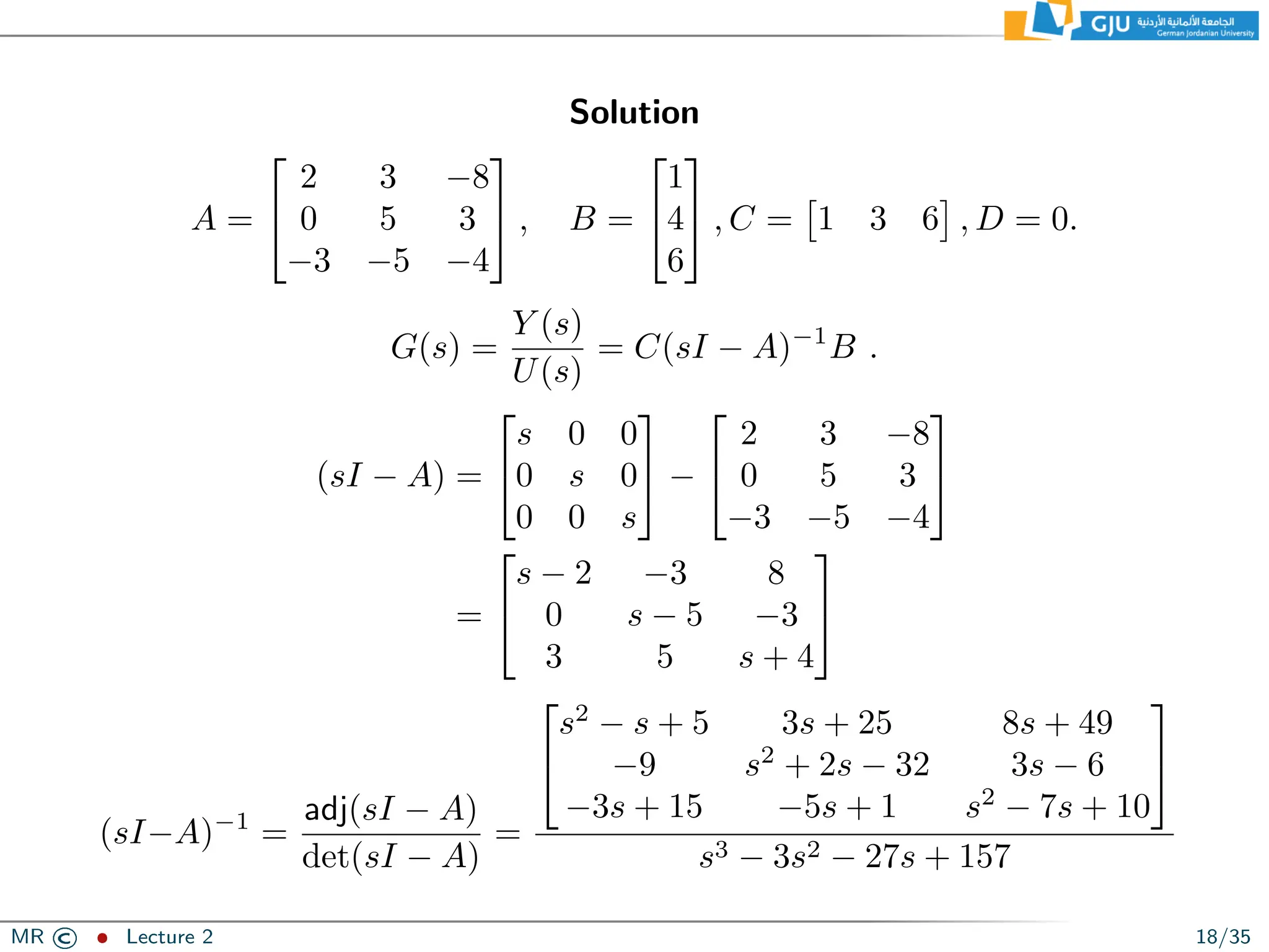
18. Solution
A =


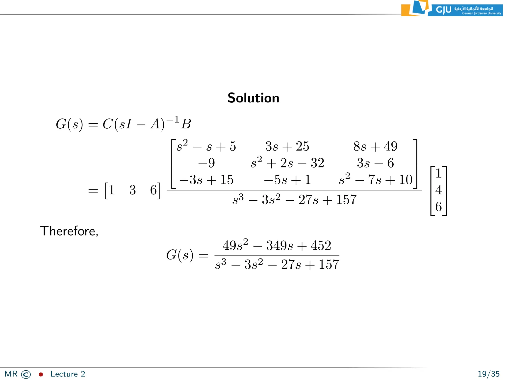
2 3 −8
0 5 3
−3 −5 −4

 , B =


1
4
6

 , C =
1 3 6
, D = 0.
G(s) =
Y (s)
U(s)
= C(sI − A)−1
B .
(sI − A) =


s 0 0
0 s 0
0 0 s

 −


2 3 −8
0 5 3
−3 −5 −4


=


s − 2 −3 8
0 s − 5 −3
3 5 s + 4


(sI−A)−1
=
adj(sI − A)
det(sI − A)
=


s2
− s + 5 3s + 25 8s + 49
−9 s2
+ 2s − 32 3s − 6
−3s + 15 −5s + 1 s2
− 7s + 10


s3 − 3s2 − 27s + 157
MR © ˆ Lecture 2 18/35

19. Solution
G(s) = C(sI − A)−1
B
=
1 3 6


s2
− s + 5 3s + 25 8s + 49
−9 s2
+ 2s − 32 3s − 6
−3s + 15 −5s + 1 s2
− 7s + 10


s3 − 3s2 − 27s + 157


1
4
6


Therefore,
G(s) =
49s2
− 349s + 452
s3 − 3s2 − 27s + 157
MR © ˆ Lecture 2 19/35

20. 3.7 Linearization
MR © ˆ Lecture 2 20/35

21. Linearization
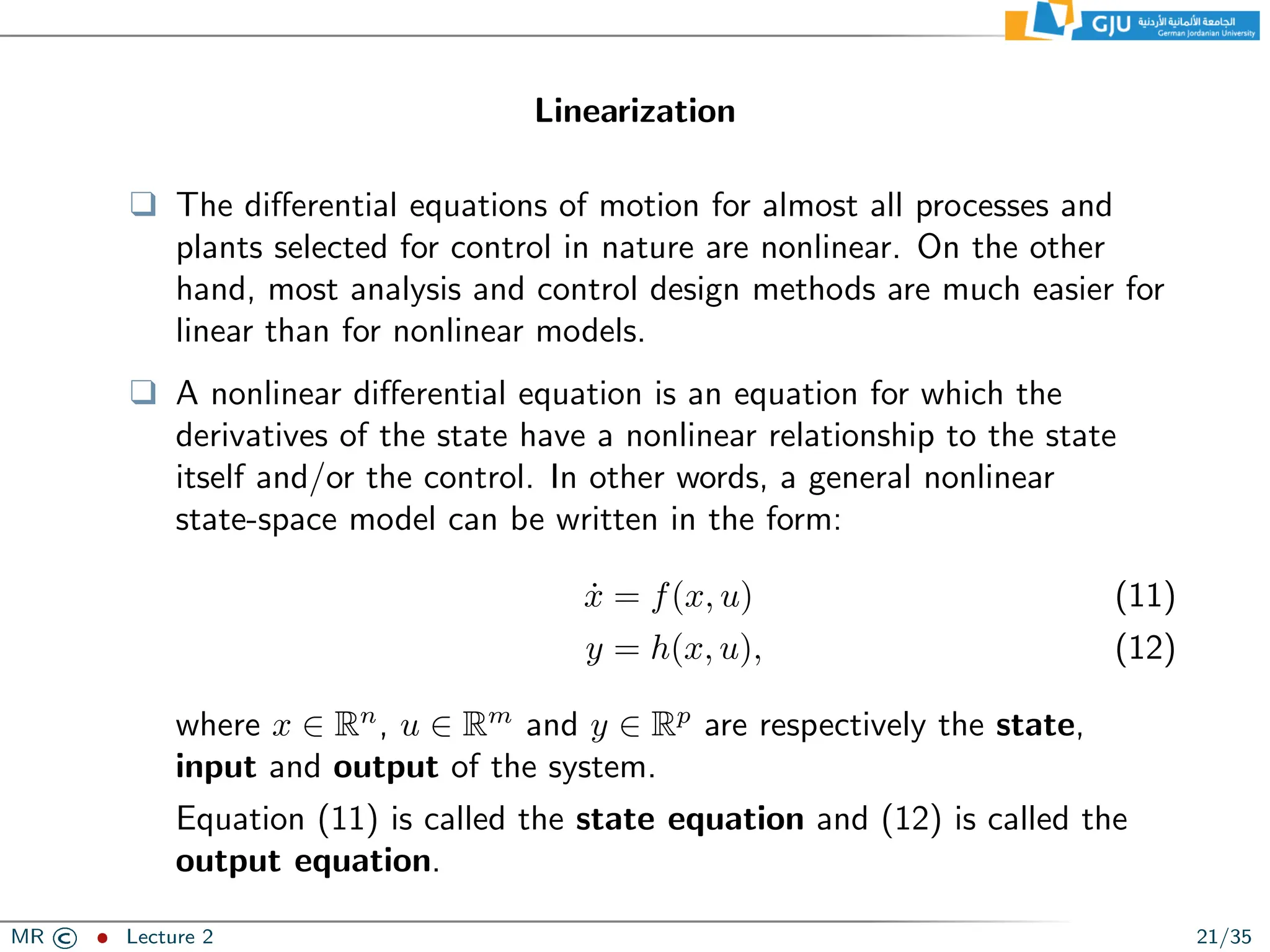
❑ The differential equations of motion for almost all processes and
plants selected for control in nature are nonlinear. On the other
hand, most analysis and control design methods are much easier for
linear than for nonlinear models.
❑ A nonlinear differential equation is an equation for which the
derivatives of the state have a nonlinear relationship to the state
itself and/or the control. In other words, a general nonlinear
state-space model can be written in the form:
ẋ = f(x, u) (11)
y = h(x, u), (12)
where x ∈ Rn
, u ∈ Rm
and y ∈ Rp
are respectively the state,
input and output of the system.
Equation (11) is called the state equation and (12) is called the
output equation.
MR © ˆ Lecture 2 21/35

22. Equilibria and Linearization
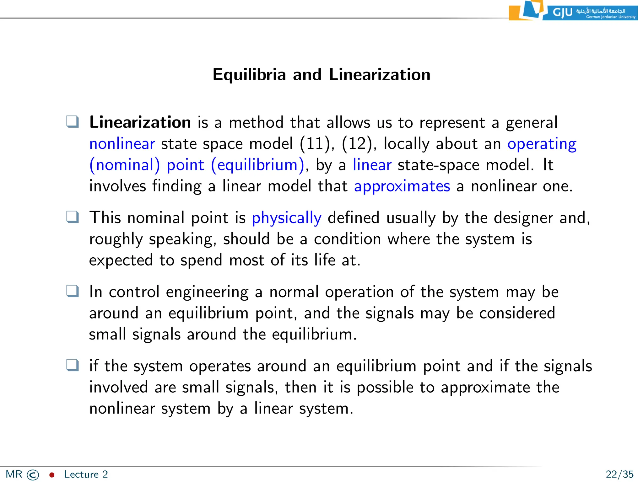
❑ Linearization is a method that allows us to represent a general
nonlinear state space model (11), (12), locally about an operating
(nominal) point (equilibrium), by a linear state-space model. It
involves finding a linear model that approximates a nonlinear one.
❑ This nominal point is physically defined usually by the designer and,
roughly speaking, should be a condition where the system is
expected to spend most of its life at.
❑ In control engineering a normal operation of the system may be
around an equilibrium point, and the signals may be considered
small signals around the equilibrium.
❑ if the system operates around an equilibrium point and if the signals
involved are small signals, then it is possible to approximate the
nonlinear system by a linear system.
MR © ˆ Lecture 2 22/35

23. Equilibria and Linearization
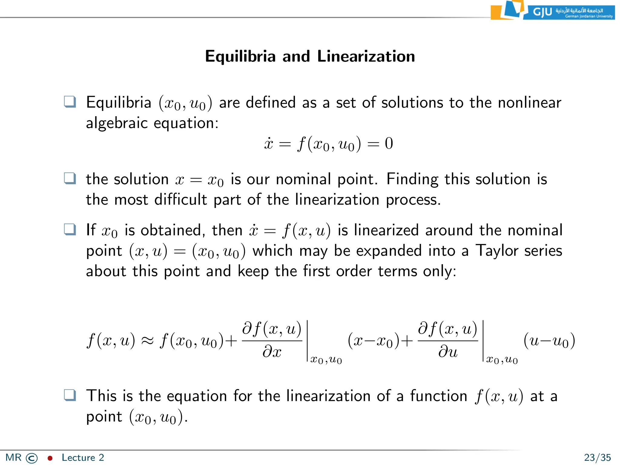
❑ Equilibria (x0, u0) are defined as a set of solutions to the nonlinear
algebraic equation:
ẋ = f(x0, u0) = 0
❑ the solution x = x0 is our nominal point. Finding this solution is
the most difficult part of the linearization process.
❑ If x0 is obtained, then ẋ = f(x, u) is linearized around the nominal
point (x, u) = (x0, u0) which may be expanded into a Taylor series
about this point and keep the first order terms only:
f(x, u) ≈ f(x0, u0)+
∂f(x, u)
∂x x0,u0
(x−x0)+
∂f(x, u)
∂u x0,u0
(u−u0)
❑ This is the equation for the linearization of a function f(x, u) at a
point (x0, u0).
MR © ˆ Lecture 2 23/35

24. ❑ Introduce new variables δx = x − x0 and δu = u − u0.
❑ Expand the nonlinear equation into McLaurin series around the
equilibrium and keep only the first order terms:
ẋ0 + δẋ ≈ f(x0, u0) + Aδx + Bδu,
where A and B are Jacobians of f with respect to x and u,
evaluated at (x0, u0), that is:
A =
∂f
∂x
(x0, u0); B =
∂f
∂u
(x0, u0)
I.e. the elements of A and B are given by:
A = [aij], where [aij] =
∂fi
∂xj
,
B = [bij], where [bij] =
∂fi
∂uj
.
❑ The system:
δẋ = Aδx + Bδu, (13)
is called the linearization of the nonlinear model ẋ = f(x, u) at
(x0, u0).
MR © ˆ Lecture 2 24/35

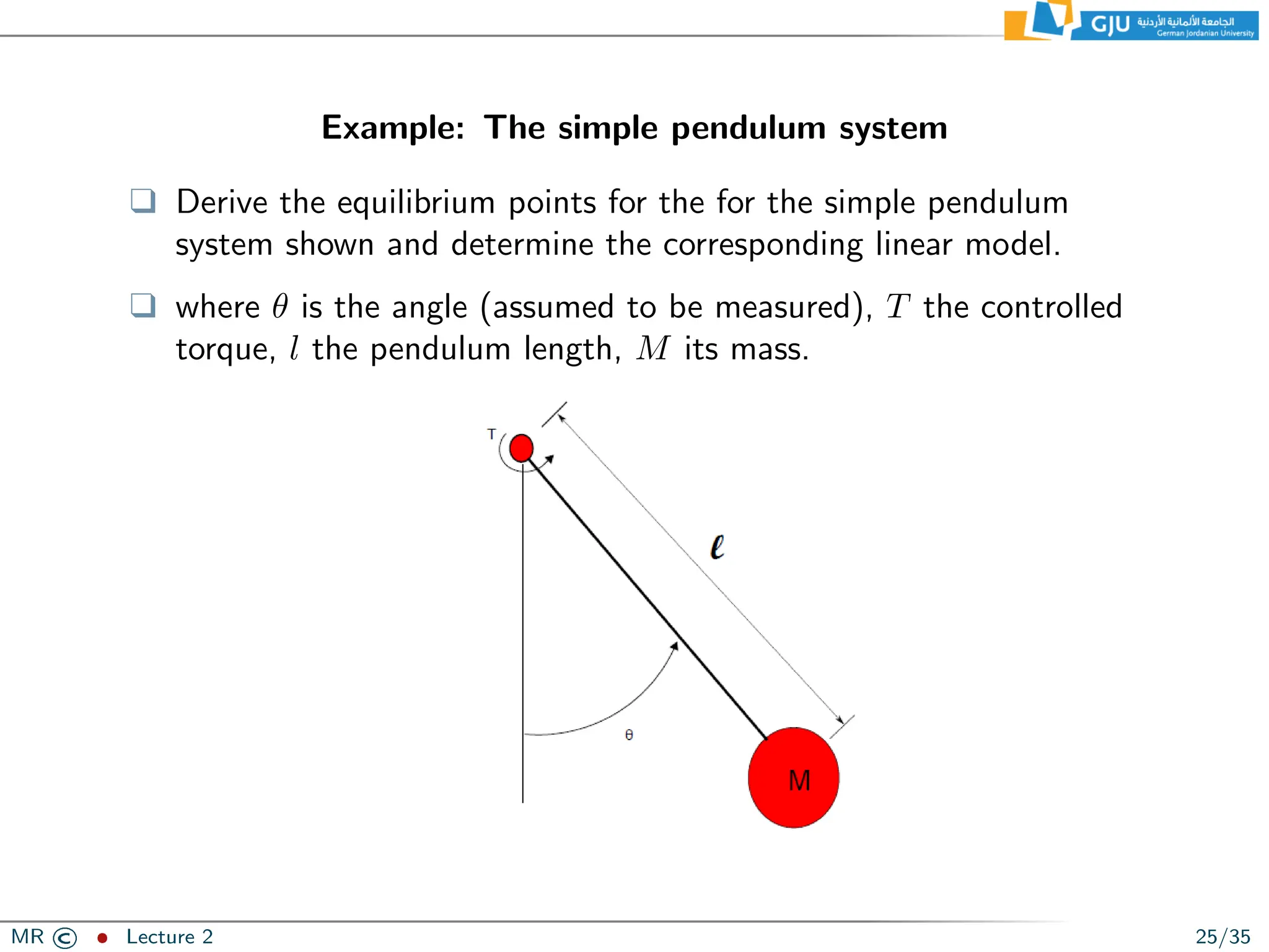
25. Example: The simple pendulum system
❑ Derive the equilibrium points for the for the simple pendulum
system shown and determine the corresponding linear model.
❑ where θ is the angle (assumed to be measured), T the controlled
torque, l the pendulum length, M its mass.
MR © ˆ Lecture 2 25/35

26. Solution
❑ First write the equations of motion , where all the mass is
concentrated at the end point and there is a torque, Tc, applied at
the pivot.
❑ Equations of motion: The moment of inertia about the pivot point
is I = ml2
❑ The sum of moments about the pivot point contains a term from
gravity as well as the applied torque T
❑ The the nonlinear equations of motion of the simple pendulum:
ΣM = Iα where α = θ̈
T − mgl sin(θ) = Iθ̈
❑ which is usually written in the form
θ̈ +
g
l
sin(θ) =
T
ml2
❑ This equation is nonlinear due to the sin(θ) term.
MR © ˆ Lecture 2 26/35

27. Solution: linearization
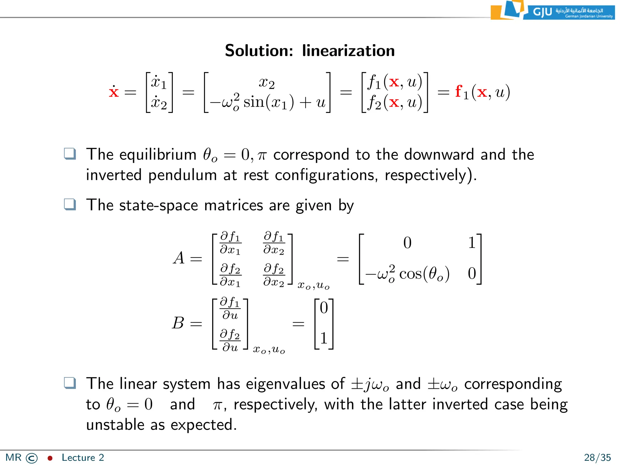
❑ First, select as state variables
x1 = θ
x2 = θ̇.
❑ The equation of motion in in state-variable form is:
ẋ =
ẋ1
ẋ2
=
x2
−ω2
o sin(x1) + u
=
f1(x, u)
f2(x, u)
= f1(x, u)
❑ where ωo =
pg
l , u = T
ml2 .
❑ To determine the equilibrium state, suppose that the (normalized)
input torque has a nominal value of uo = 0. Then
ẋ1 = x2 = 0 =⇒ x2 = 0
ẋ2 = −ω2
o sin(x1) = 0, =⇒ sin(x1) = 0
❑ sin(x1 = θ) = 0 =⇒ θo = 0, π.
MR © ˆ Lecture 2 27/35

28. Solution: linearization
ẋ =
ẋ1
ẋ2
=
x2
−ω2
o sin(x1) + u
=
f1(x, u)
f2(x, u)
= f1(x, u)
❑ The equilibrium θo = 0, π correspond to the downward and the
inverted pendulum at rest configurations, respectively).
❑ The state-space matrices are given by
A =
∂f1
∂x1
∂f1
∂x2
∂f2
∂x1
∂f2
∂x2
#
xo,uo
=
0 1
−ω2
o cos(θo) 0
#
B =
∂f1
∂u
∂f2
∂u
#
xo,uo
=
0
1
#
❑ The linear system has eigenvalues of ±jωo and ±ωo corresponding
to θo = 0 and π, respectively, with the latter inverted case being
unstable as expected.
MR © ˆ Lecture 2 28/35

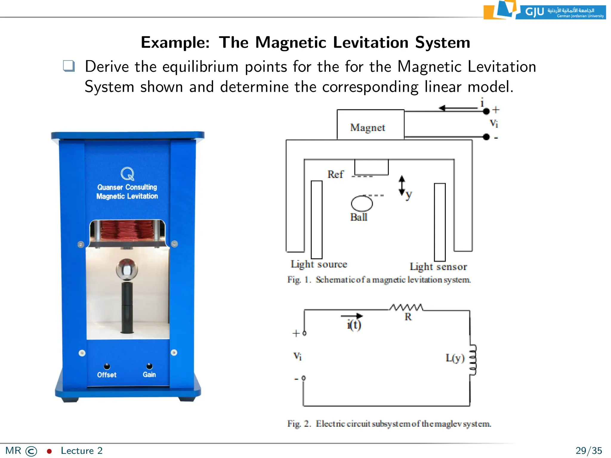
29. Example: The Magnetic Levitation System
❑ Derive the equilibrium points for the for the Magnetic Levitation
System shown and determine the corresponding linear model.
MR © ˆ Lecture 2 29/35

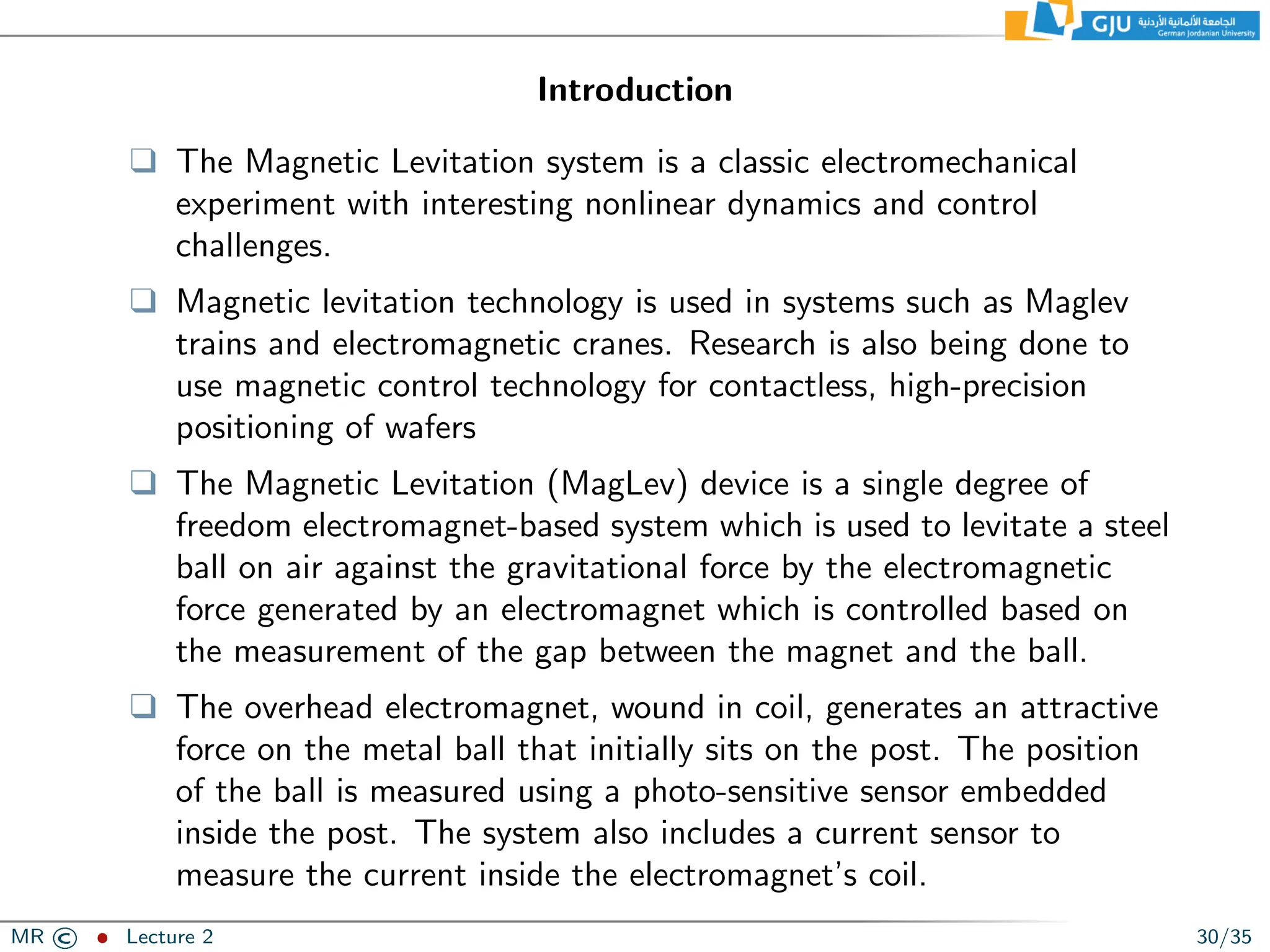
30. Introduction
❑ The Magnetic Levitation system is a classic electromechanical
experiment with interesting nonlinear dynamics and control
challenges.
❑ Magnetic levitation technology is used in systems such as Maglev
trains and electromagnetic cranes. Research is also being done to
use magnetic control technology for contactless, high-precision
positioning of wafers
❑ The Magnetic Levitation (MagLev) device is a single degree of
freedom electromagnet-based system which is used to levitate a steel
ball on air against the gravitational force by the electromagnetic
force generated by an electromagnet which is controlled based on
the measurement of the gap between the magnet and the ball.
❑ The overhead electromagnet, wound in coil, generates an attractive
force on the metal ball that initially sits on the post. The position
of the ball is measured using a photo-sensitive sensor embedded
inside the post. The system also includes a current sensor to
measure the current inside the electromagnet’s coil.
MR © ˆ Lecture 2 30/35

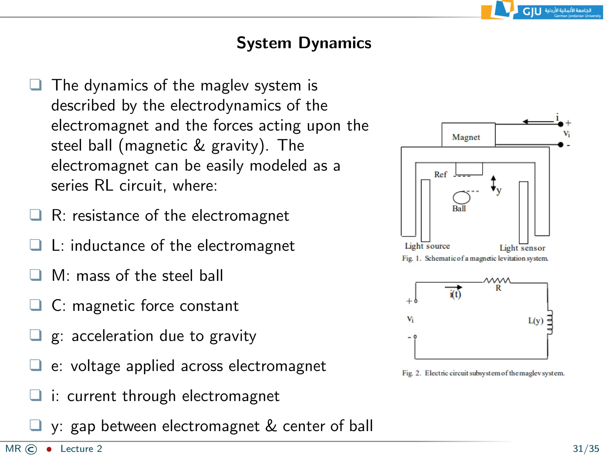
31. System Dynamics
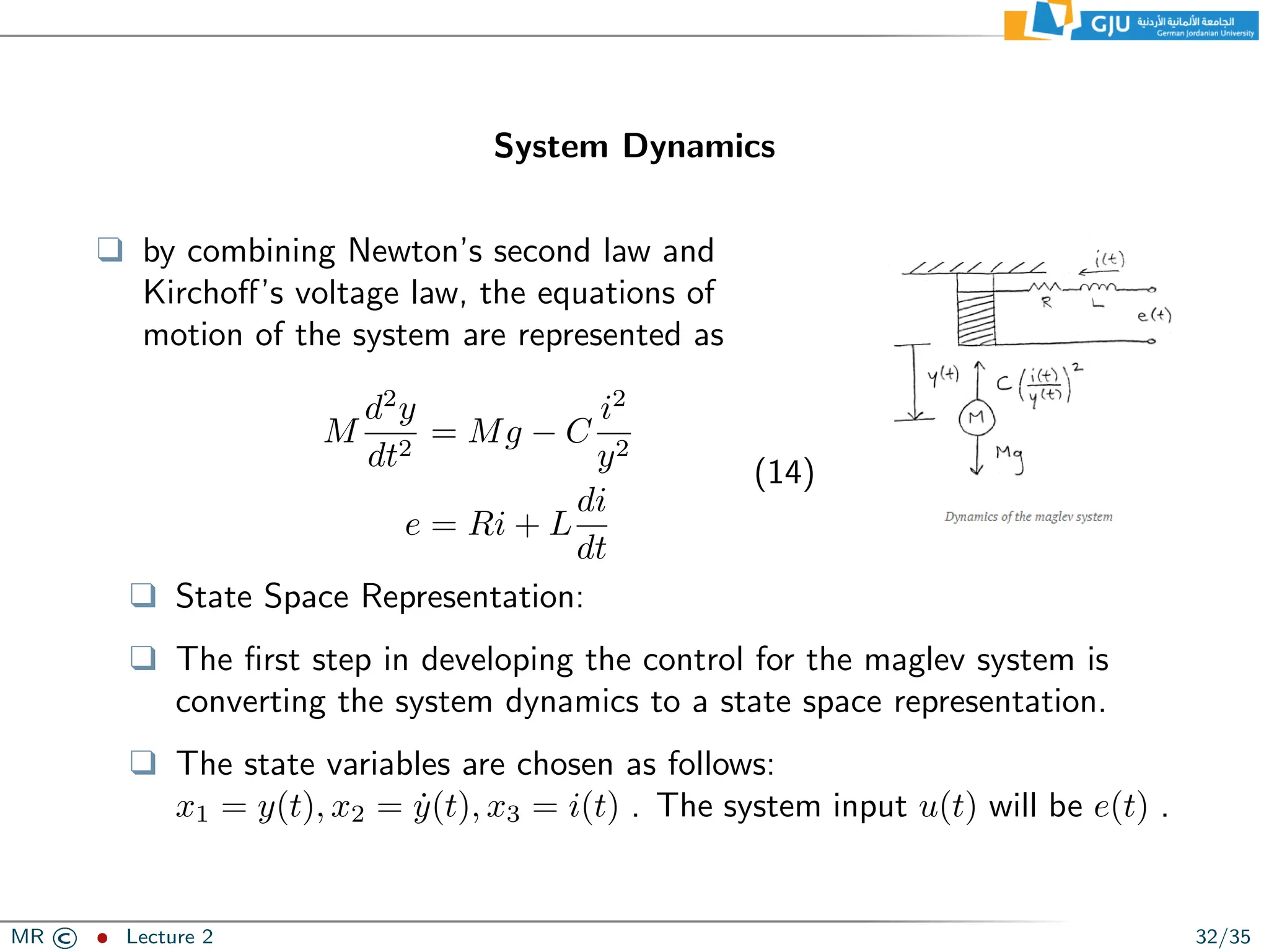
❑ The dynamics of the maglev system is
described by the electrodynamics of the
electromagnet and the forces acting upon the
steel ball (magnetic gravity). The
electromagnet can be easily modeled as a
series RL circuit, where:
❑ R: resistance of the electromagnet
❑ L: inductance of the electromagnet
❑ M: mass of the steel ball
❑ C: magnetic force constant
❑ g: acceleration due to gravity
❑ e: voltage applied across electromagnet
❑ i: current through electromagnet
❑ y: gap between electromagnet center of ball
MR © ˆ Lecture 2 31/35

32. System Dynamics
❑ by combining Newton’s second law and
Kirchoff’s voltage law, the equations of
motion of the system are represented as
M
d2
y
dt2
= Mg − C
i2
y2
e = Ri + L
di
dt
(14)
❑ State Space Representation:
❑ The first step in developing the control for the maglev system is
converting the system dynamics to a state space representation.
❑ The state variables are chosen as follows:
x1 = y(t), x2 = ẏ(t), x3 = i(t) . The system input u(t) will be e(t) .
MR © ˆ Lecture 2 32/35

33. System Dynamics
❑ Expressing the system dynamics in terms of the state variables
yields the following equations
ẋ1 = x2
ẋ2 = g −
C
M
x3
x1
2
ẋ3 =
1
L
(u − Rx3)
(15)
with f = [ẋ1, ẋ2, ẋ3]T
and ẋ = [x1, x2, x3]T
.
❑ Clearly, the system dynamics are non-linear.
❑ it is preferable to linearize the system about an equilibrium point.
❑ The equilibrium points of a system are found by setting f = 0 and
solving for x1, x2, x3, u.
❑ Since there are four variables to solve for and only three equations,
the system is underdetermined.
MR © ˆ Lecture 2 33/35

34. Determining the Equilibrium Point
❑ This can be remedied by setting x1(t) = d , where d (desired) is the
height set point.
❑ Solving for the variables yields the following equilibrium point
❑ (Note: we are interested in the equilibrium point (e) corresponding
to levitation of the steel ball. The equilibrium point corresponding
to x3 = 0 is not of interest since this implies the electromagnet is
turned off).
x1,e = d
x2,e = 0
x3,e = d
r
Mg
C
ue = dR
r
Mg
C
(16)
with f(xe) = [x1,e, x2,e, x3,e]T
.
MR © ˆ Lecture 2 34/35

35. Linearizing the System Dynamics
❑ The linearized system describes the system dynamics relative to the
equilibrium point.
❑ We define δx = x − xe and δu = u − ue as the deviations of the
state and control from the equilibrium point, respectively.
❑ The linearized system dynamics are given by
δẋ = Ãδx + B̃δu.
❑ where à = df/dx is the Jacobian of the state matrix and
B̃ = du/dx is the Jacobian of the input matrix, both evaluated at
the equilibrium point [xe, ue] .
❑ Computation of à and B̃ yields the following linear system
δẋ =



0 1 0
2g
d 0 −2
q
Cg
M
0 0 −R
L


 δx +


0
0
1
L

 δu
MR © ˆ Lecture 2 35/35