


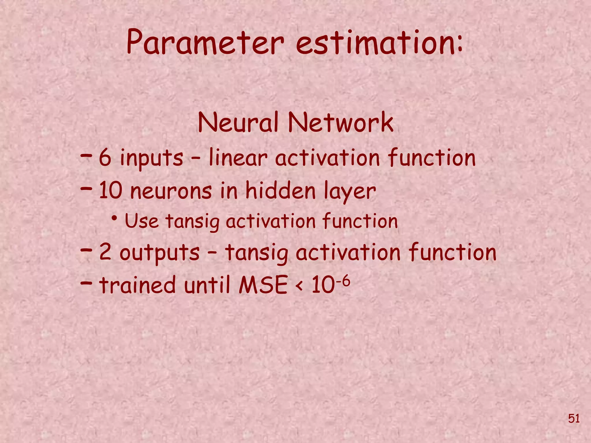
![46
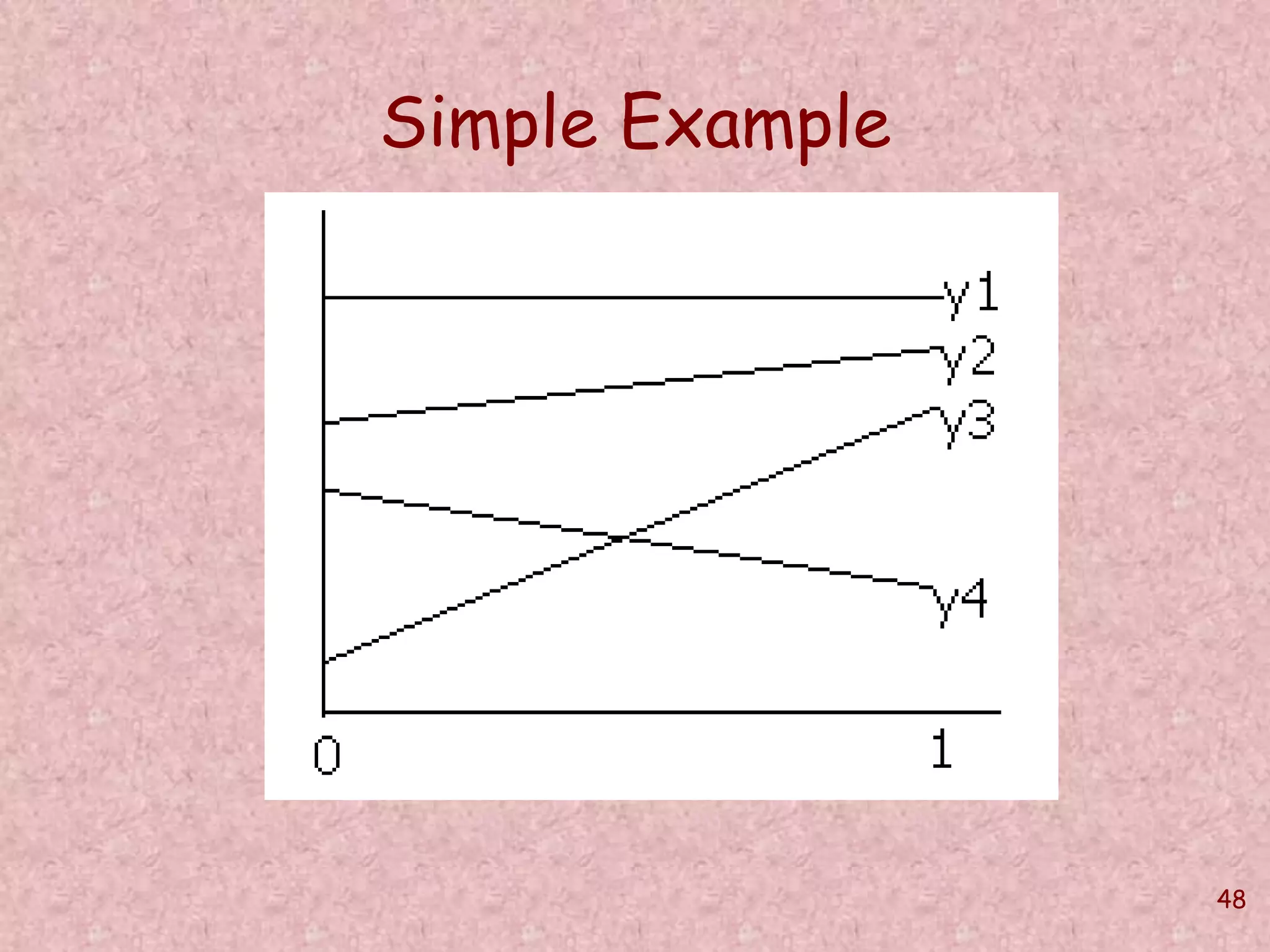
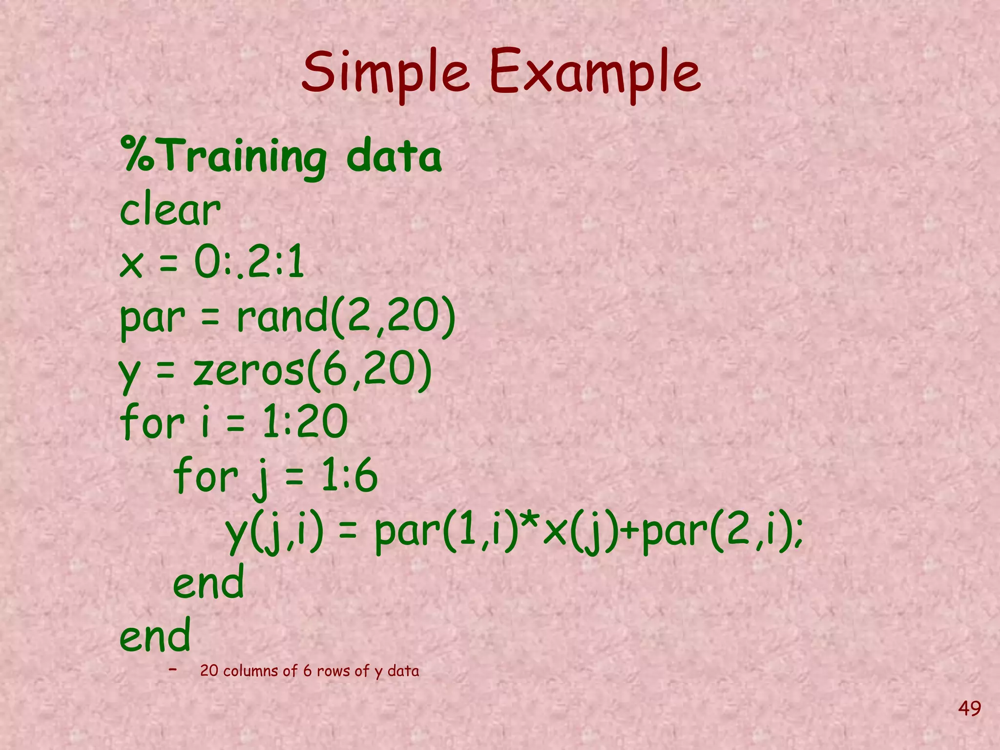
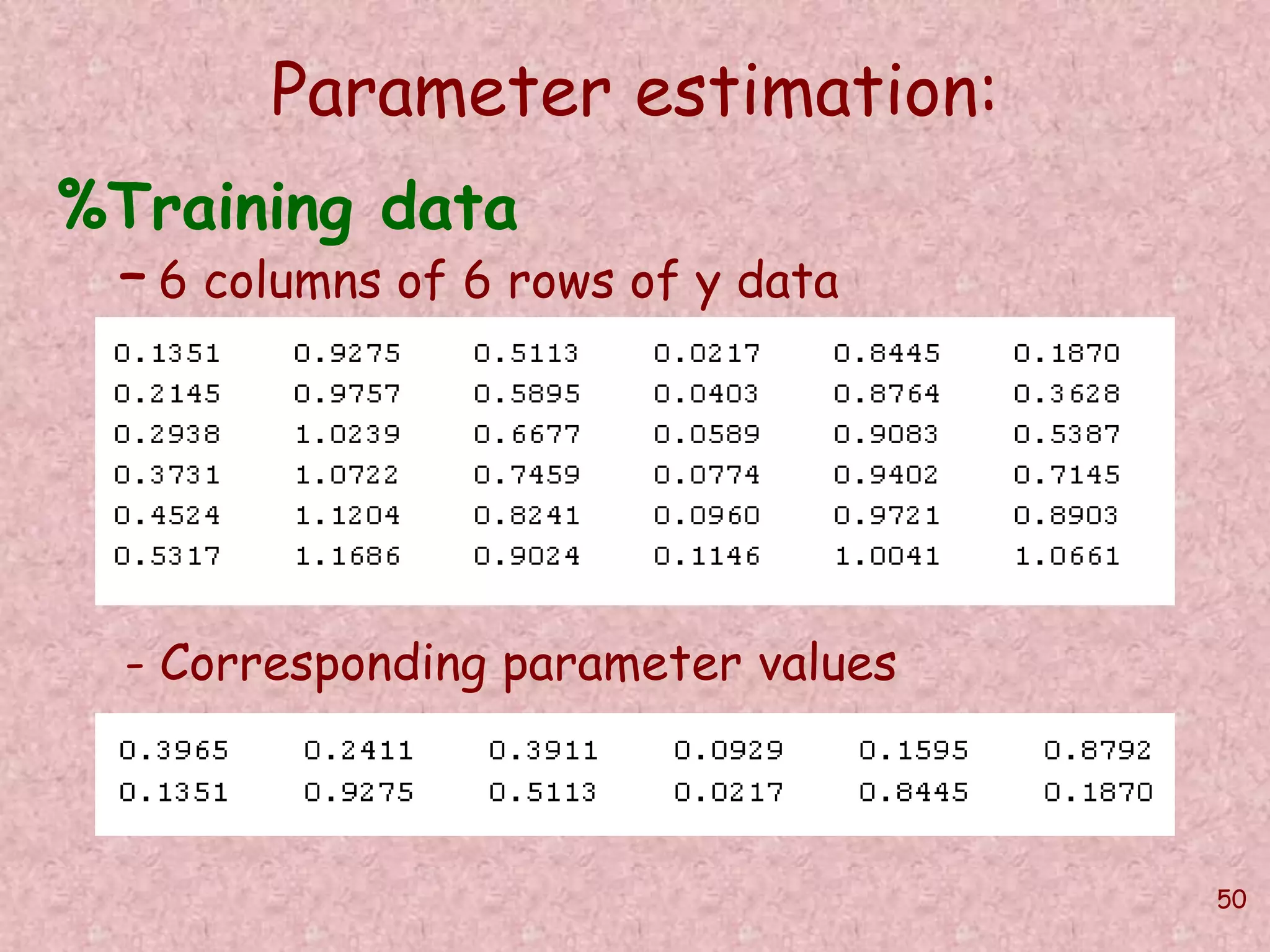
Simple Parameter Estimation
Y = mx+b
• Given a number of points on a line,
determine the slope (m) and intercept
(b) of the line
– Fix number of points at 6
– Restrict domain 0 ≤ x ≤ 1
– Restrict range of b and m to [ -1, 1 ]](https://image.slidesharecdn.com/softcomputingpkp-140918044704-phpapp01/75/Soft-computing-ANN-and-Fuzzy-Logic-Dr-Purnima-Pandit-46-2048.jpg)
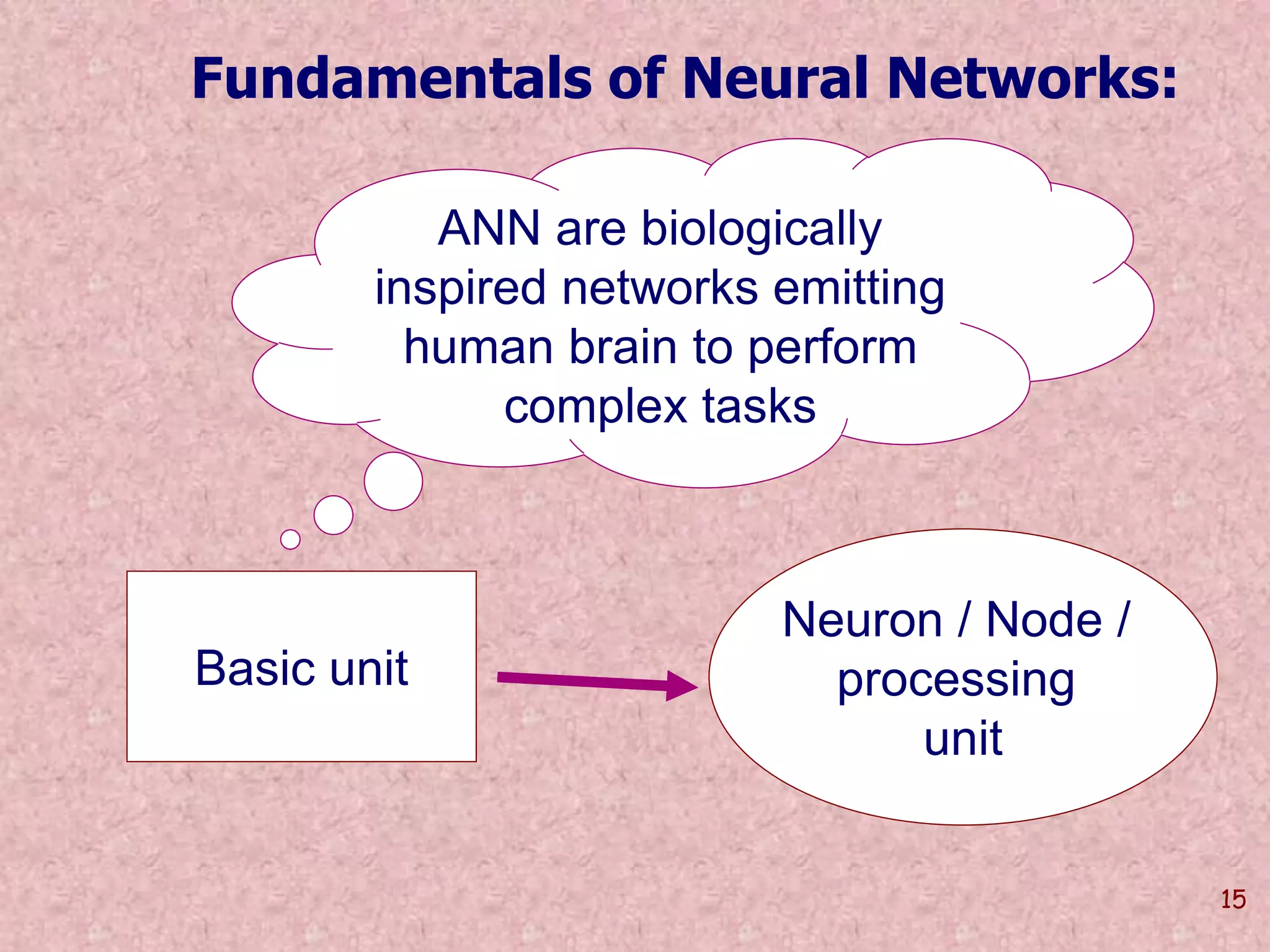
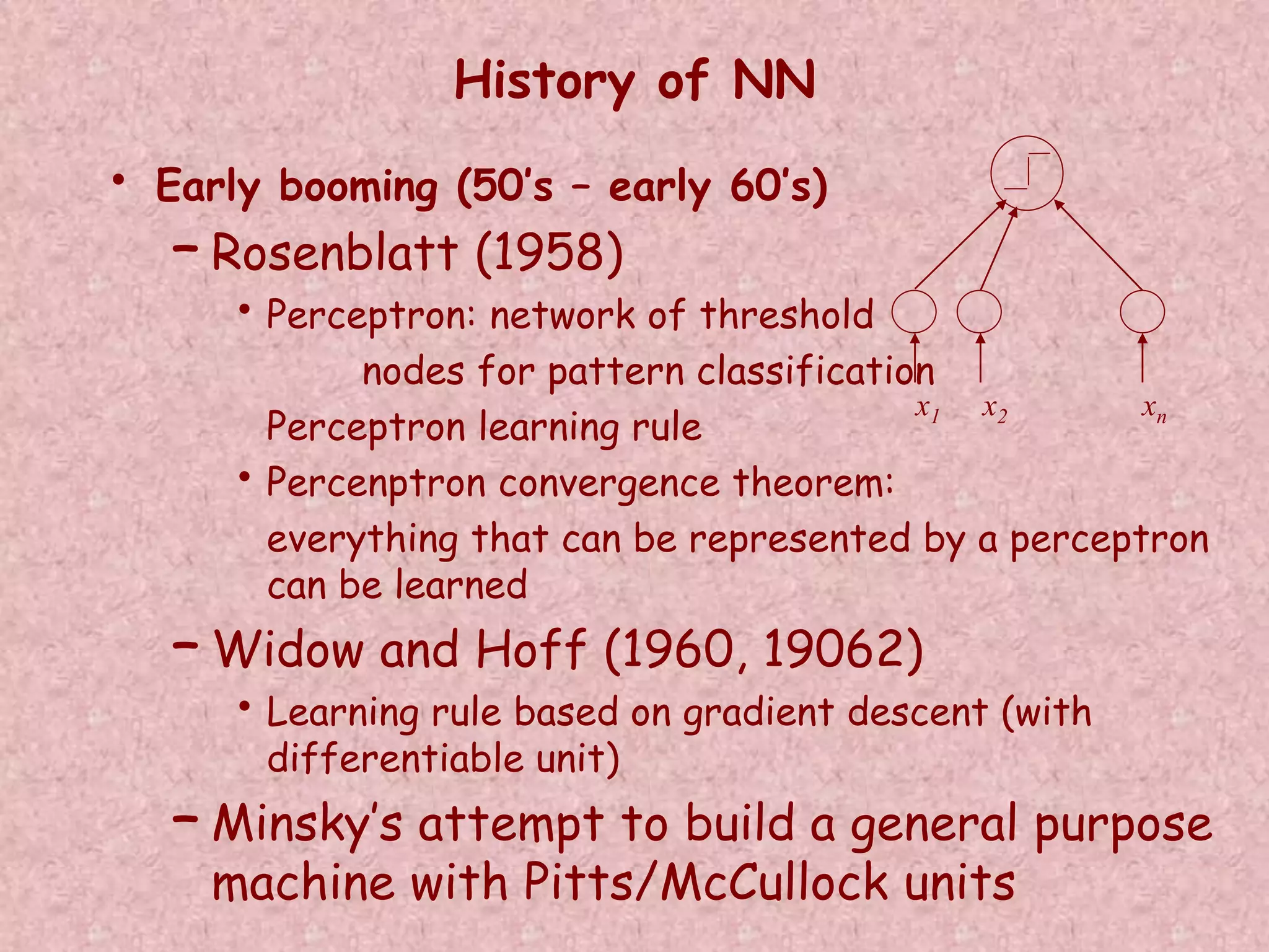
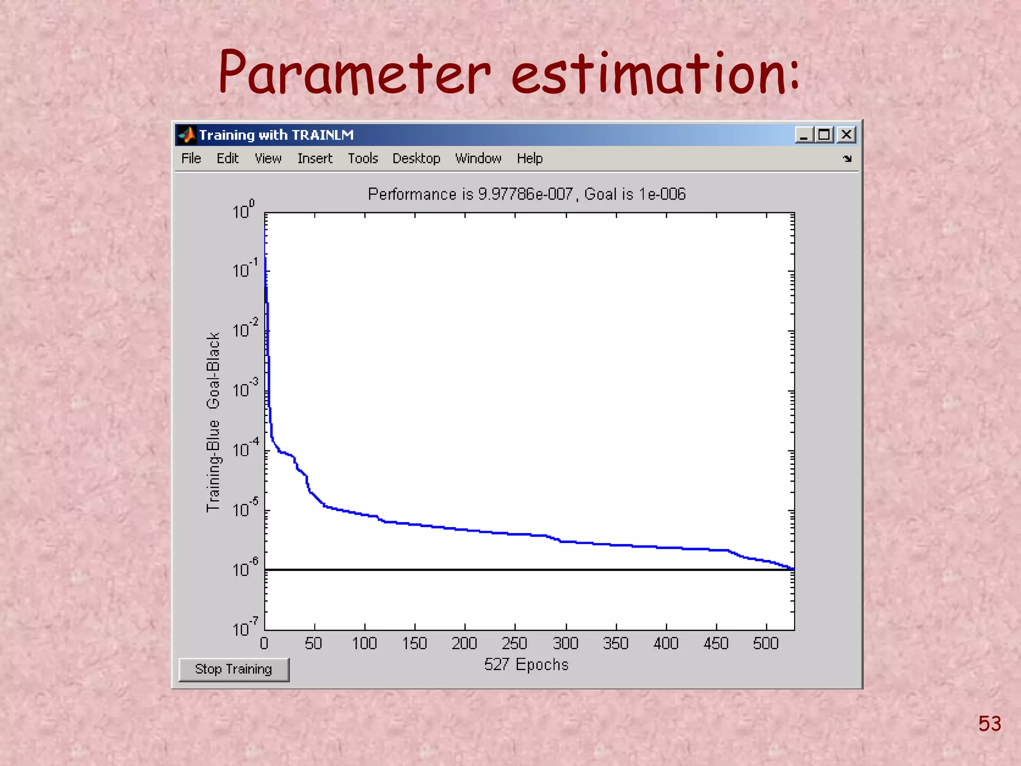
![52
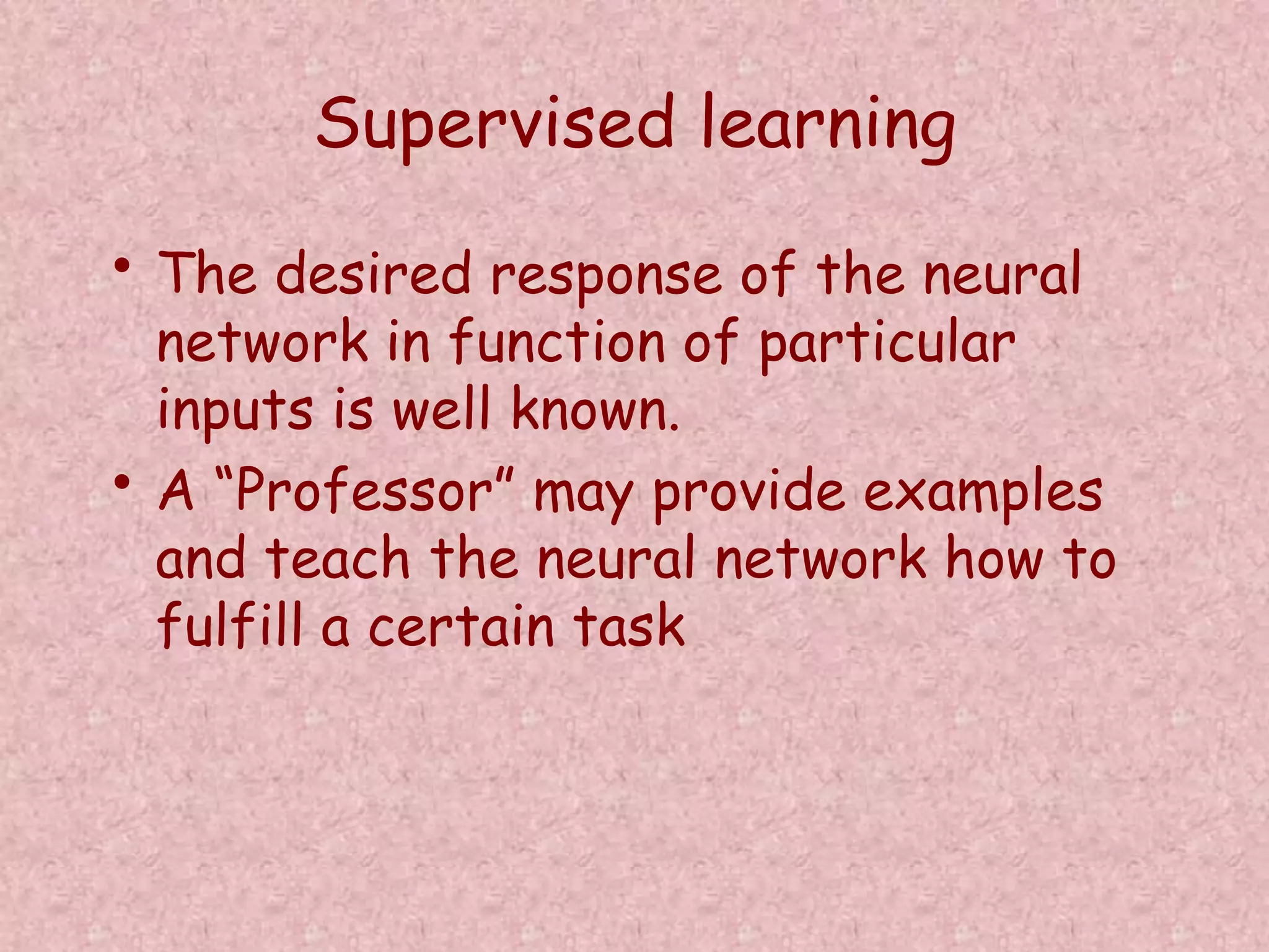
Parameter estimation:
netu = newff([0 1;0 1;0 1;0 1;0 1; 0 1],[10,
2],{'tansig' 'tansig'}, 'trainlm', 'learngdm',
'mse');
netu = init(netu);
Pu = y;
Tu = par;
netu.trainParam.epochs = 100000;
netu.trainParam.goal = 0.000001;
netu = train(netu,Pu,Tu);
yu = sim(netu,Pu)](https://image.slidesharecdn.com/softcomputingpkp-140918044704-phpapp01/75/Soft-computing-ANN-and-Fuzzy-Logic-Dr-Purnima-Pandit-52-2048.jpg)
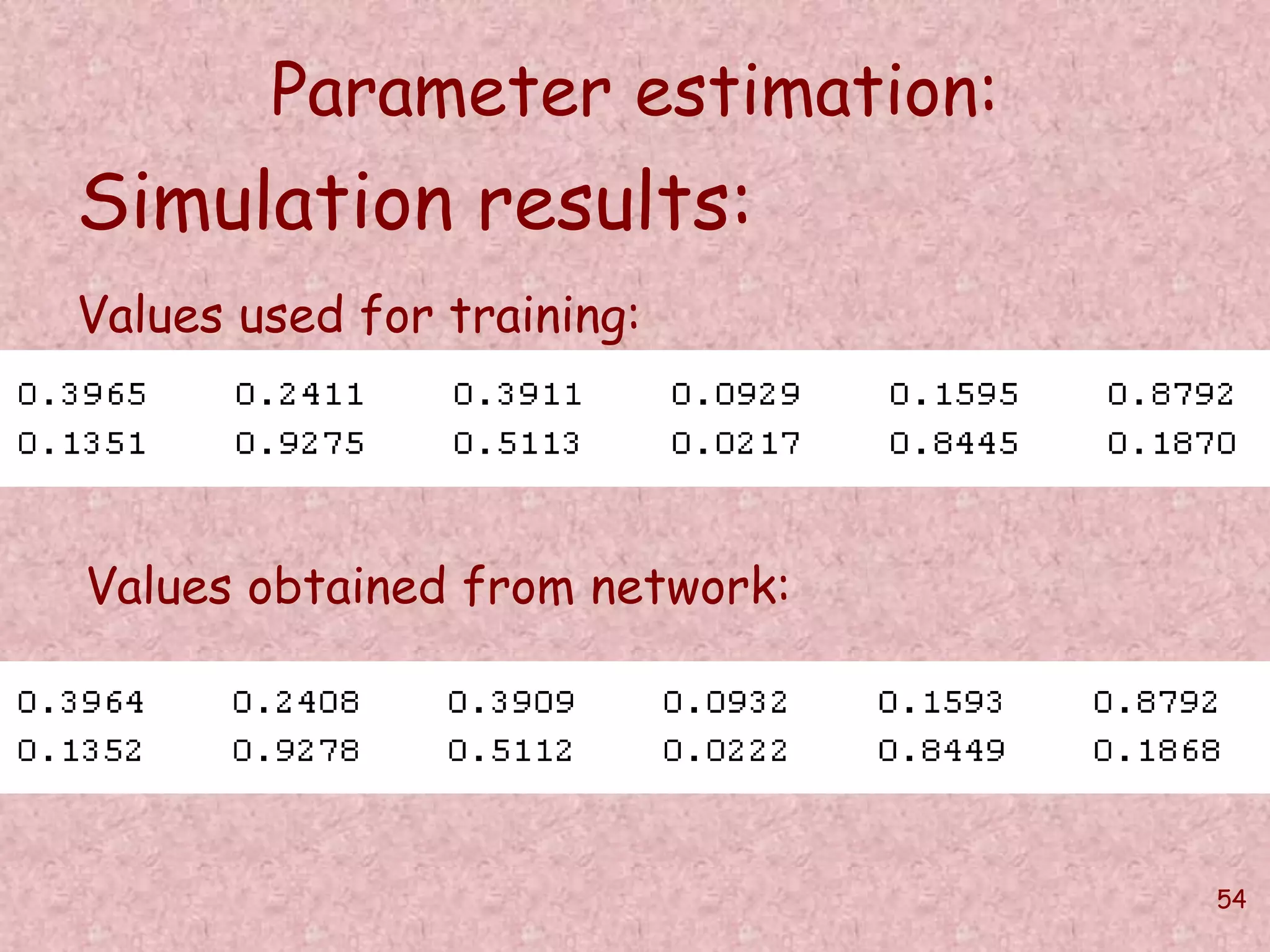
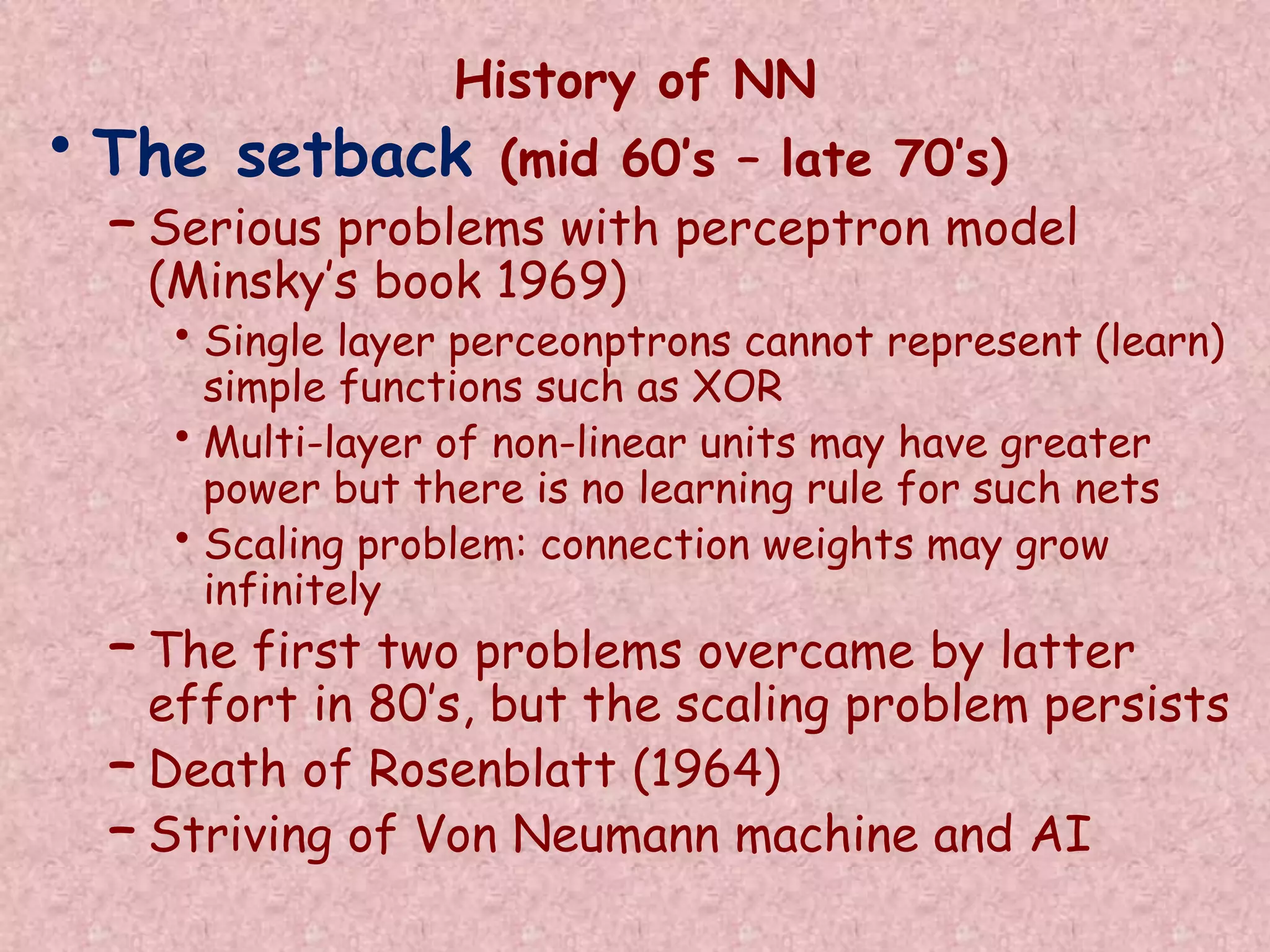
![55
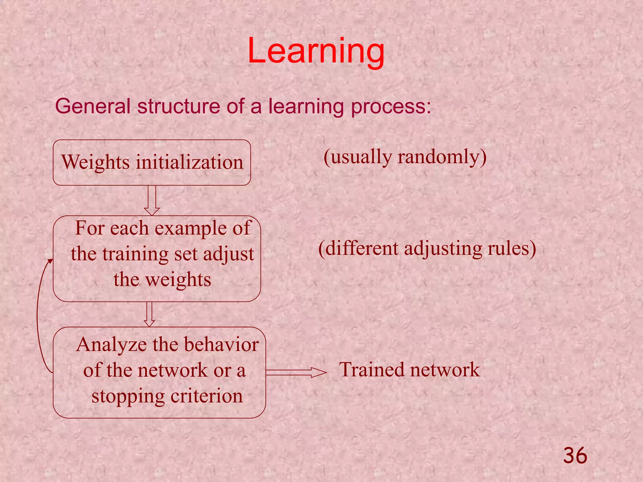
Parameter estimation:
Generalization validation:
Using parameter values
m = 0.3974 and b = 0.7316
we generate input vector:
[ 0.7316 0.8110 0.8905 0.9700 1.0495 1.1290 ]’
For this input vector the trained Neural Network
produces the output as:
0.3946
0.7323](https://image.slidesharecdn.com/softcomputingpkp-140918044704-phpapp01/75/Soft-computing-ANN-and-Fuzzy-Logic-Dr-Purnima-Pandit-55-2048.jpg)


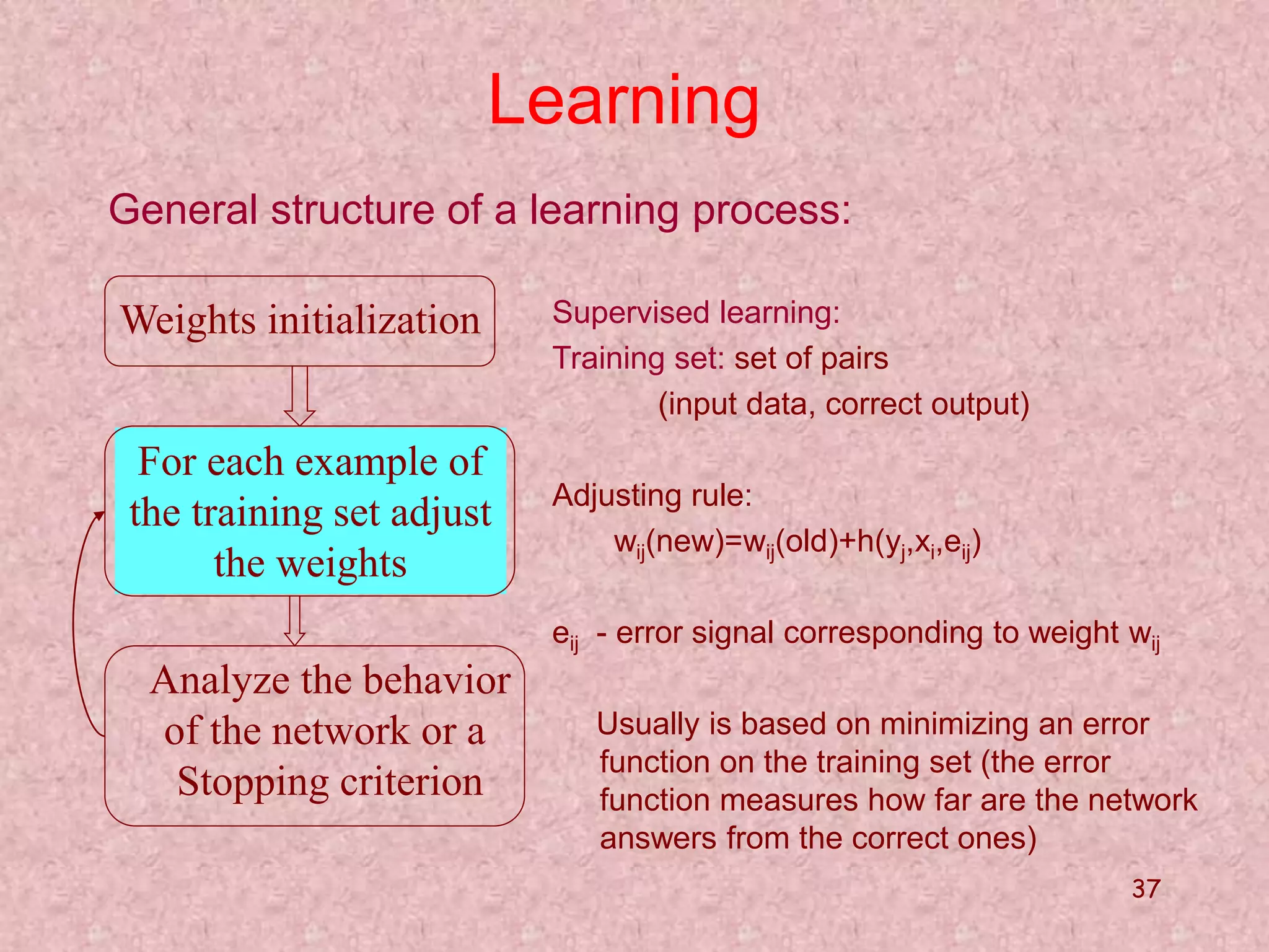
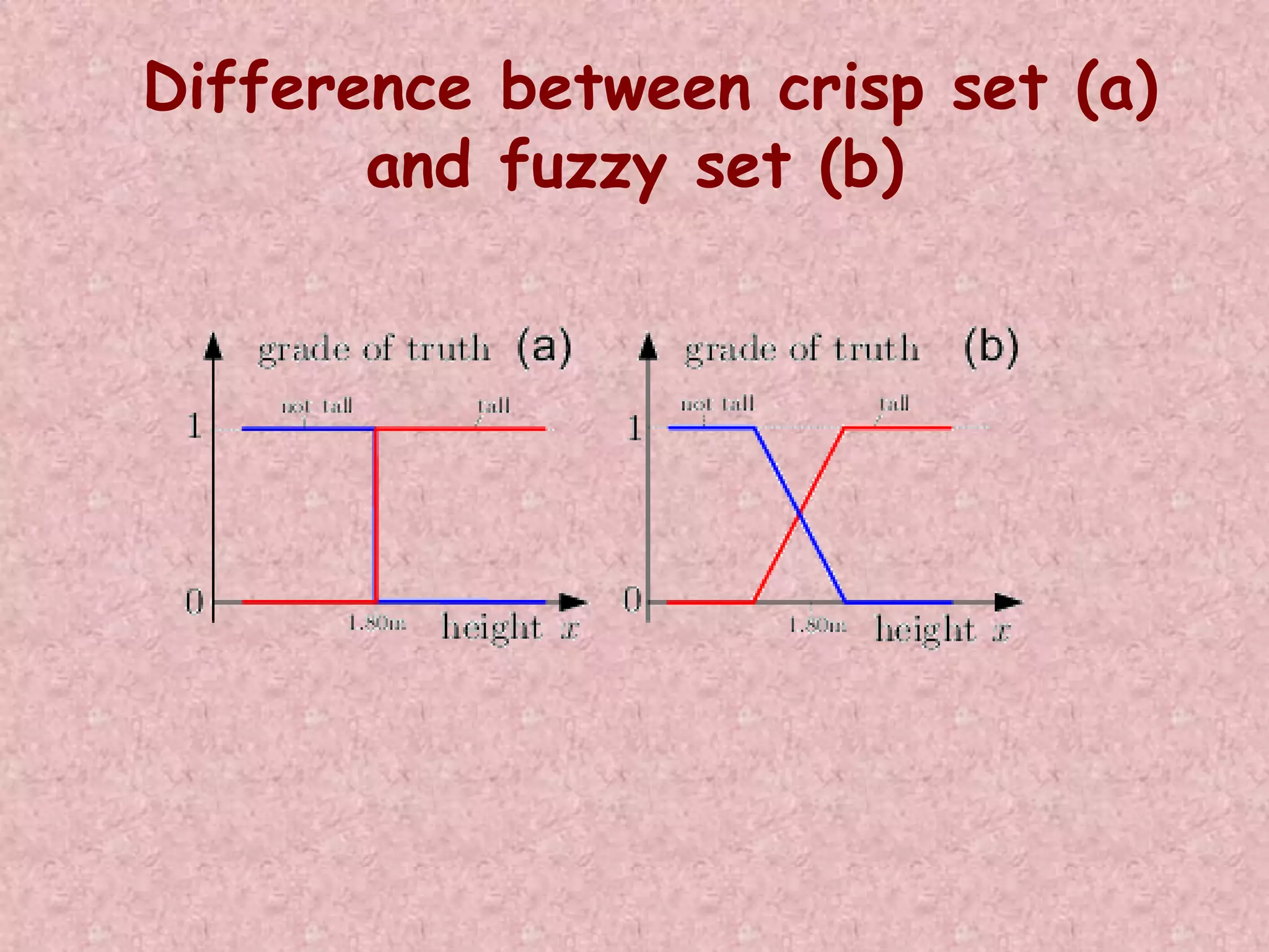
![Characteristic Function in the Case
of Crisp Sets and Fuzzy Sets
P: X {0,1}
P(x) =
A : X [0,1]
A = {X, A(x)} if x X
1 if
x X
x
X
0 if
A Fuzzy Set is a generalized set to which objects can
belongs with various degrees (grades) of memberships
over the interval [0,1].](https://image.slidesharecdn.com/softcomputingpkp-140918044704-phpapp01/75/Soft-computing-ANN-and-Fuzzy-Logic-Dr-Purnima-Pandit-66-2048.jpg)
![Operations on Fuzzy sets
• Standard complement :-
A’(x) = 1 − A(x)
• Standard intersection:-
(A ∩ B)(x) = min [A(x), B(x)]
• Standard union:-
(A U B)(x) = max [A(x), B(x)]](https://image.slidesharecdn.com/softcomputingpkp-140918044704-phpapp01/75/Soft-computing-ANN-and-Fuzzy-Logic-Dr-Purnima-Pandit-68-2048.jpg)
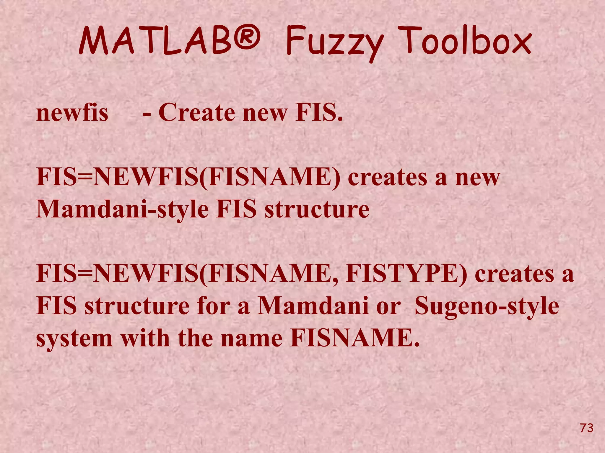
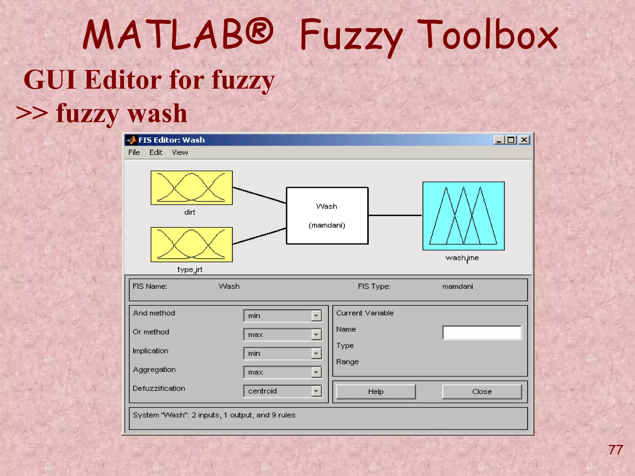
![75
MATLAB® Fuzzy Toolbox
addvar - Add variable to FIS.
w = addvar(w,varType,varName,varBounds)
w = addvar(w,'input','dirt',[0,100]);
addmf - Add membership function to FIS
w = addmf(w,varType,varIndex,mfName,
mfType, mfParams)
w = addmf(w,'input',1,'small','trimf',[-50 0 50]);](https://image.slidesharecdn.com/softcomputingpkp-140918044704-phpapp01/75/Soft-computing-ANN-and-Fuzzy-Logic-Dr-Purnima-Pandit-75-2048.jpg)
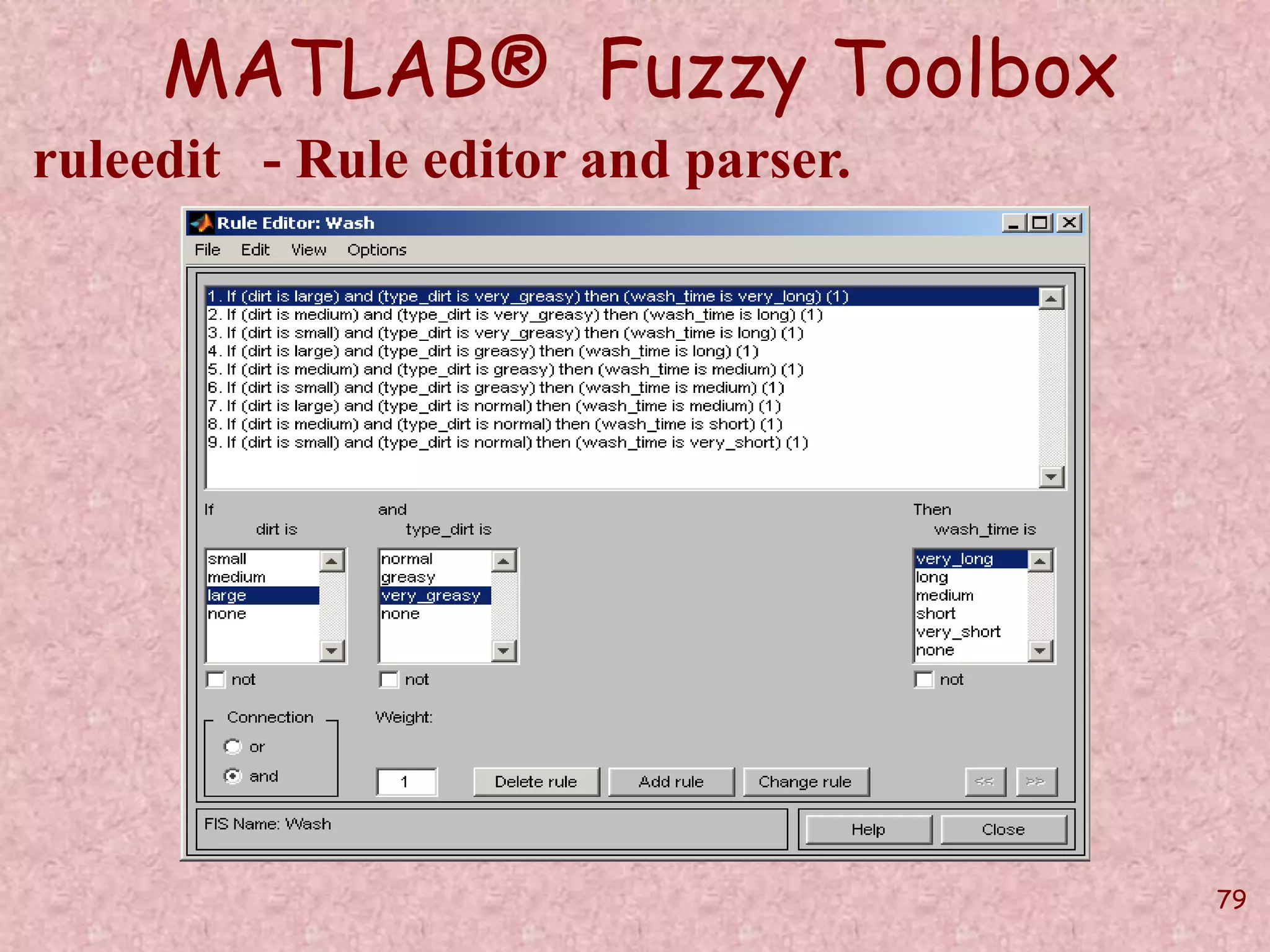
![76
MATLAB® Fuzzy Toolbox
addrule - Add rule to FIS.
ruleList=[1 1 1 1 1;
1 2 2 1 1];
w = addrule(w,ruleList);](https://image.slidesharecdn.com/softcomputingpkp-140918044704-phpapp01/75/Soft-computing-ANN-and-Fuzzy-Logic-Dr-Purnima-Pandit-76-2048.jpg)

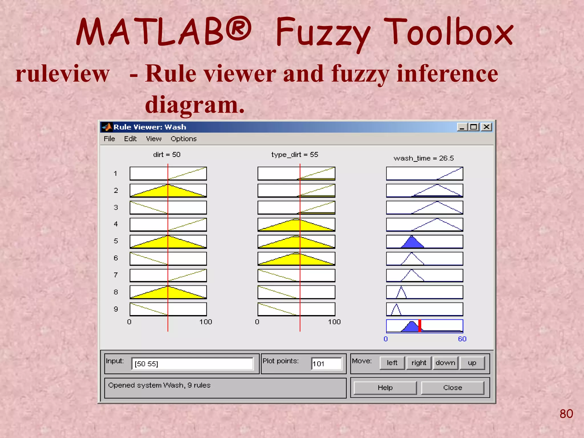
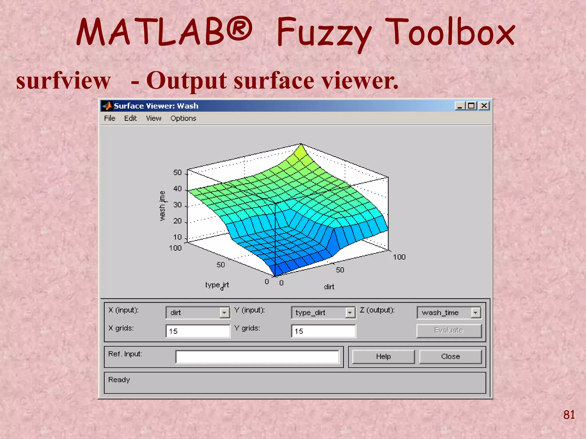
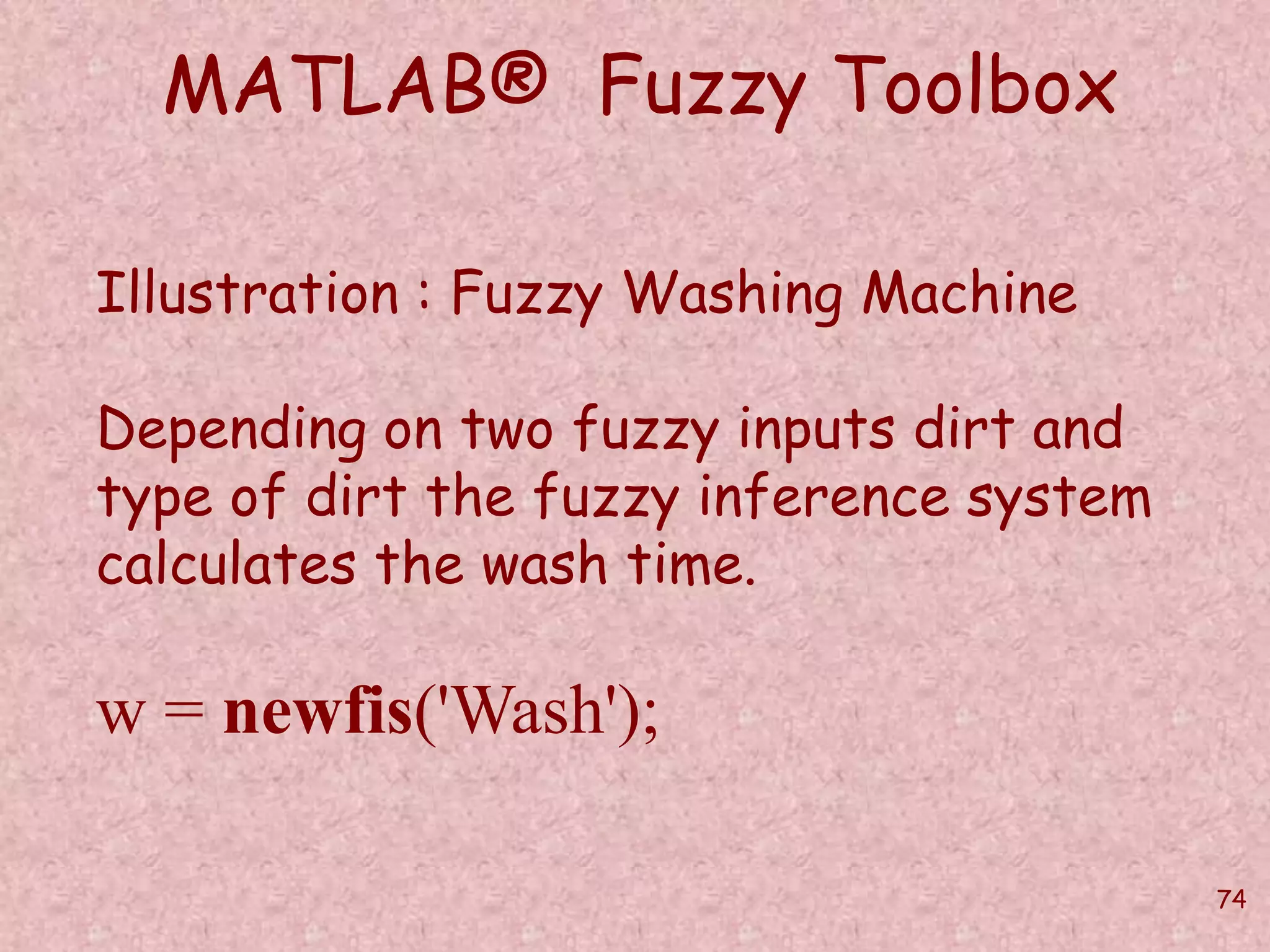
![82
MATLAB® Fuzzy Toolbox
w = newfis('Wash');
w = addvar(w,'input','dirt',[0,100]);
w = addvar(w,'input','type_dirt',[0,100]);
w = addvar(w,'output','wash_time',[0,60]);
w = addmf(w,'input',1,'small','trimf',[-50 0 50]);
w = addmf(w,'input',1,'medium','trimf',[0 50 100]);
w = addmf(w,'input',1,'large','trimf',[50 100 150]);
w = addmf(w,'input',2,'normal','trimf',[-50 0 50]);
w = addmf(w,'input',2,'greasy','trimf',[0 50 100]);
w = addmf(w,'input',2,'very_greasy','trimf',[50 100 150]);
w = addmf(w,'output',1,'very_long','trimf',[40 60 80]);
w = addmf(w,'output',1,'long','trimf',[20 40 60]);
w = addmf(w,'output',1,'medium','trimf',[12 20 30]);
w = addmf(w,'output',1,'short','trimf',[8 12 16]);
w = addmf(w,'output',1,'very_short','trimf',[4 8 12]);
ruleList = [3 3 1 1 1;2 3 2 1 1; 1 3 2 1 1; 3 2 2 1 1; 2 2 3 1 1; 1 2 3 1 1; 3 1 3 1 1;2 1 4 1 1;
1 1 5 1 1];
w = addrule(w,ruleList);
gensurf(w,[1 2]);
surfview(w)](https://image.slidesharecdn.com/softcomputingpkp-140918044704-phpapp01/75/Soft-computing-ANN-and-Fuzzy-Logic-Dr-Purnima-Pandit-82-2048.jpg)


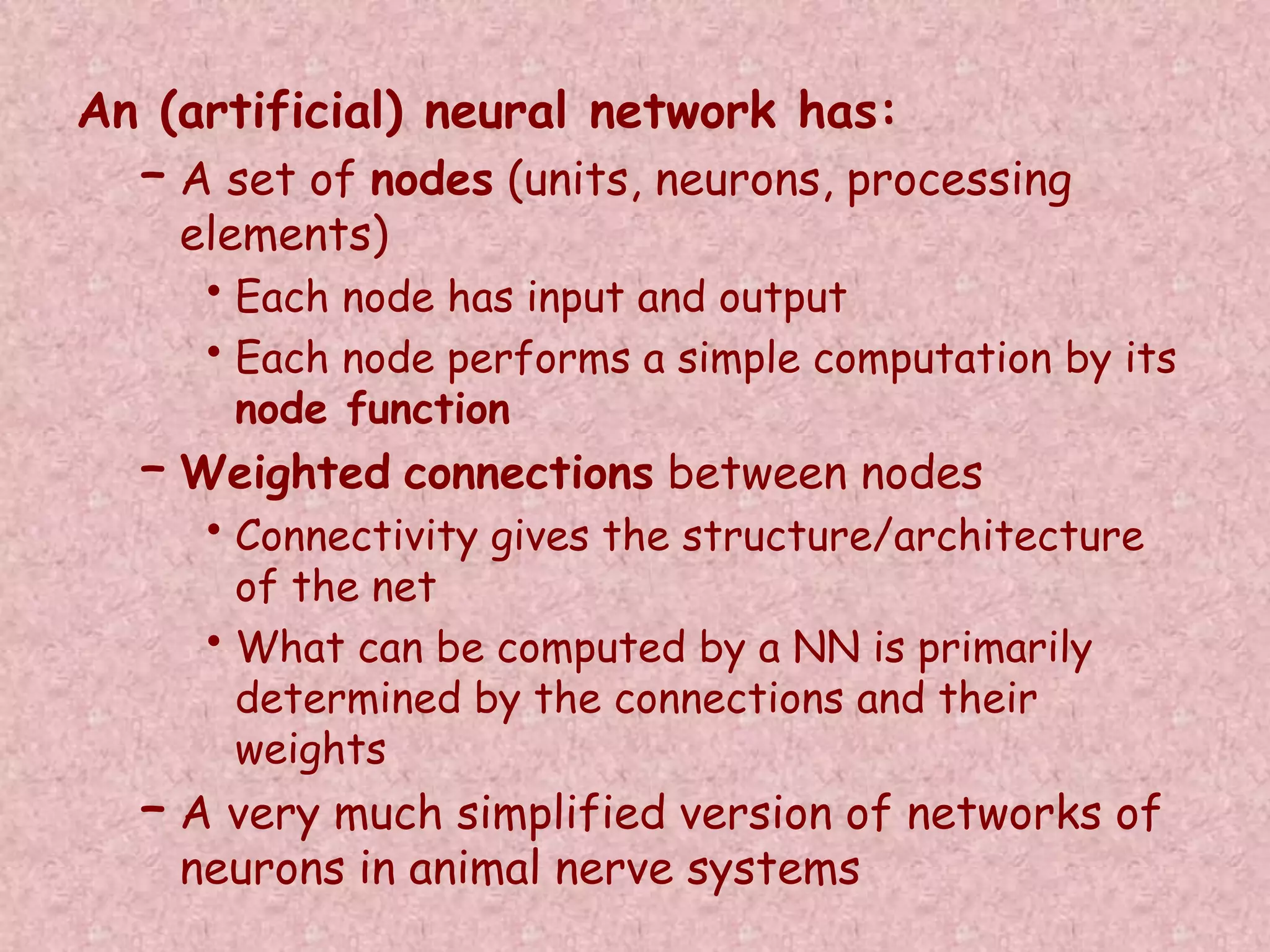
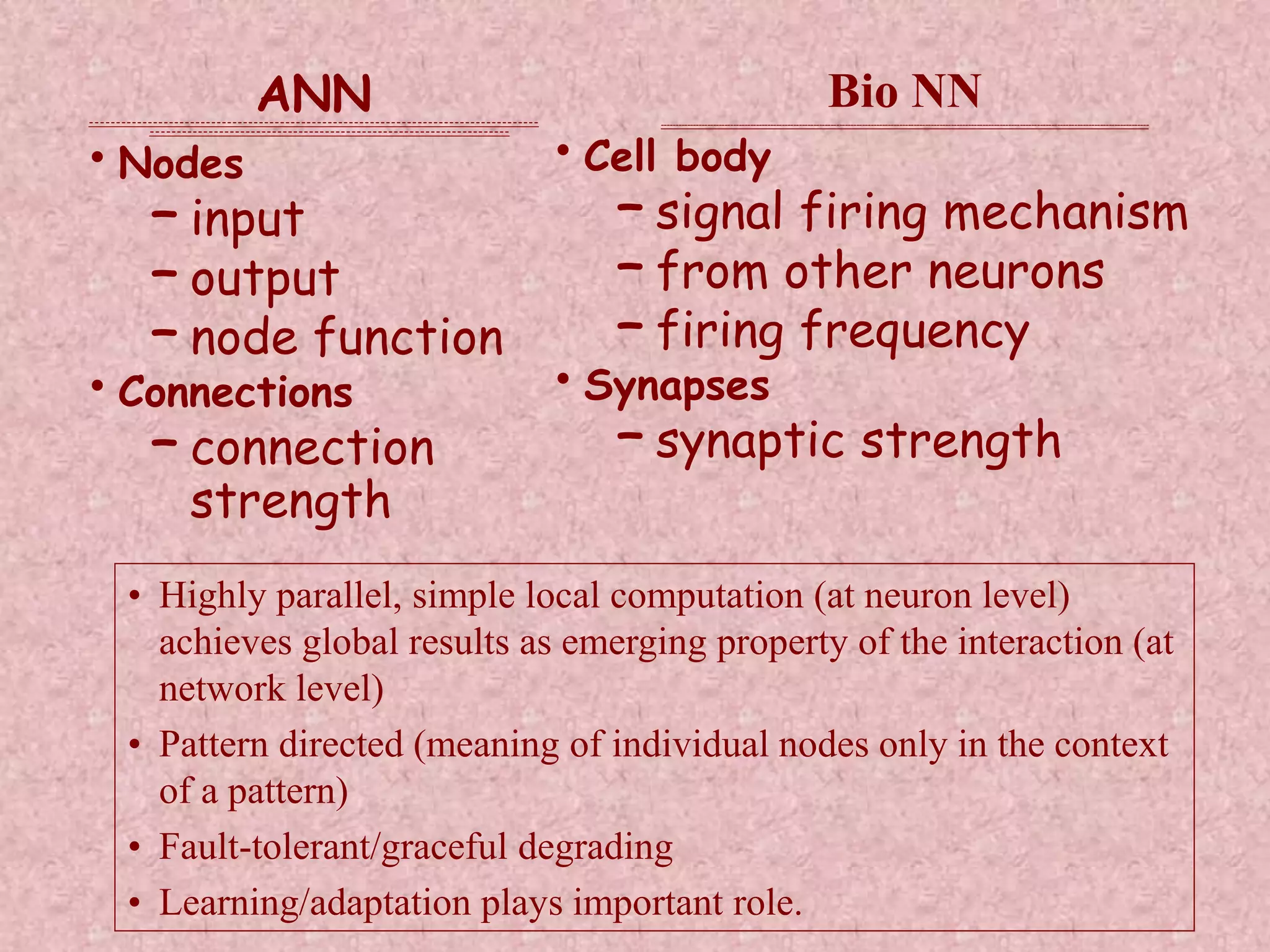
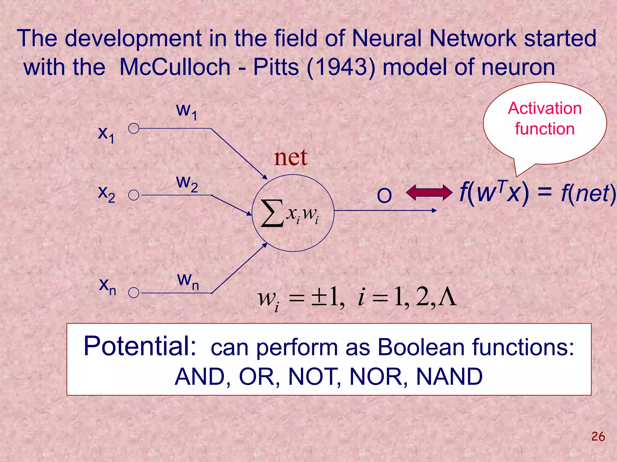
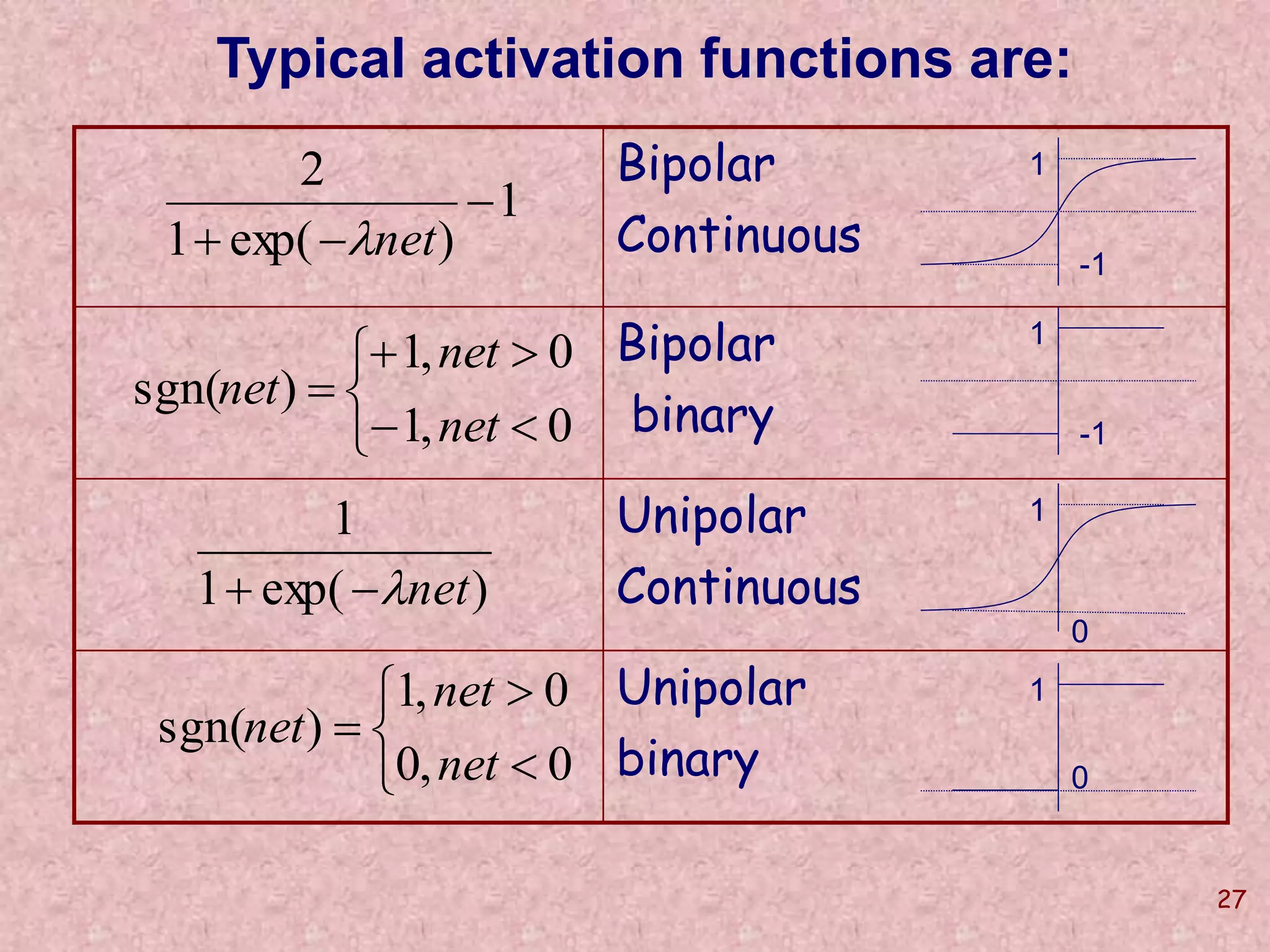
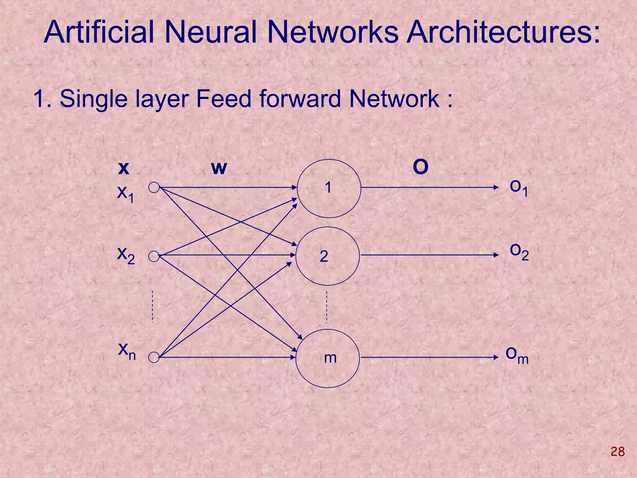
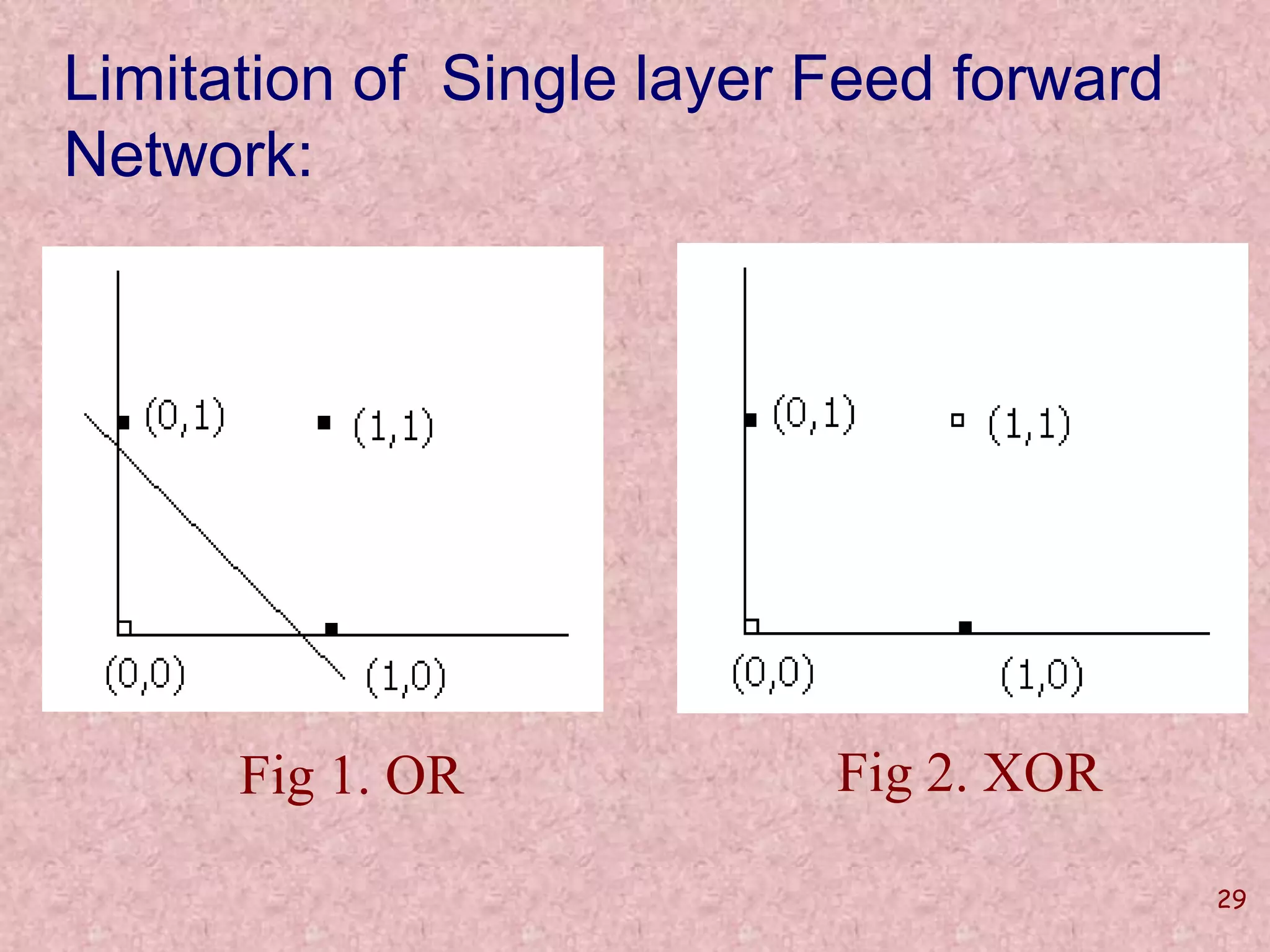
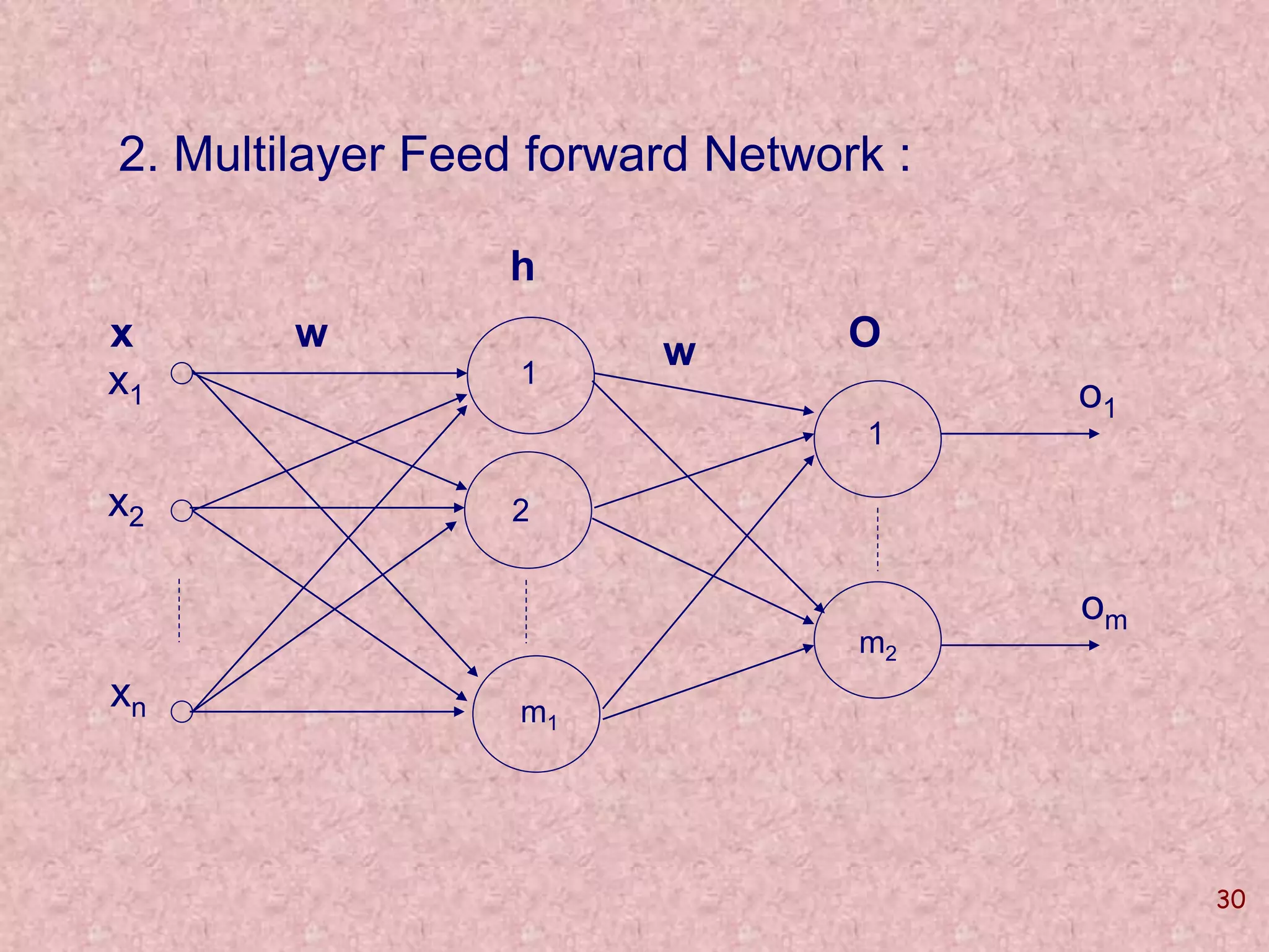
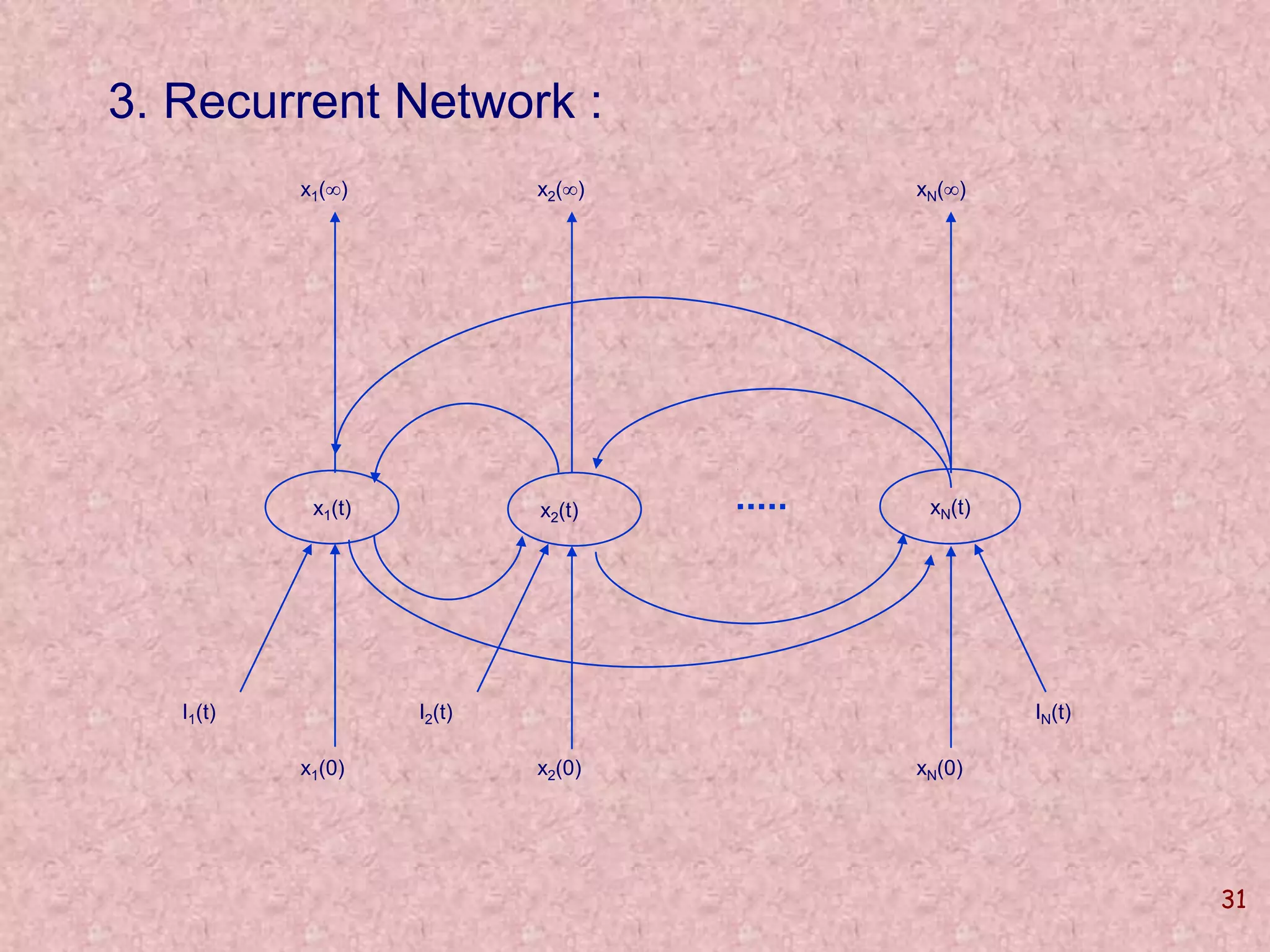
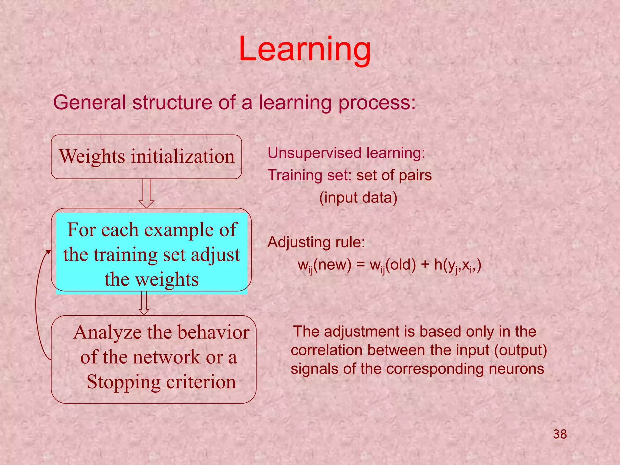
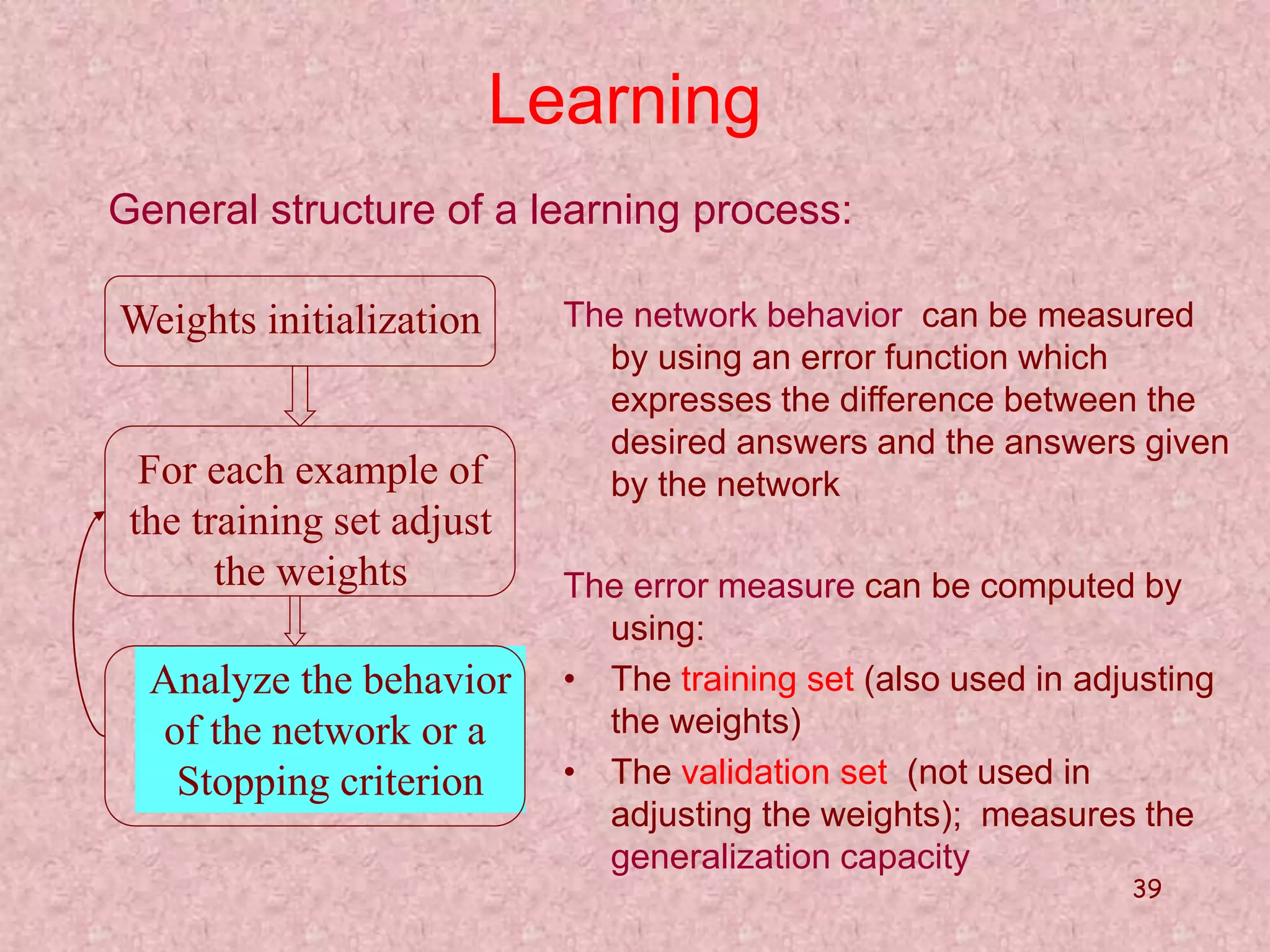
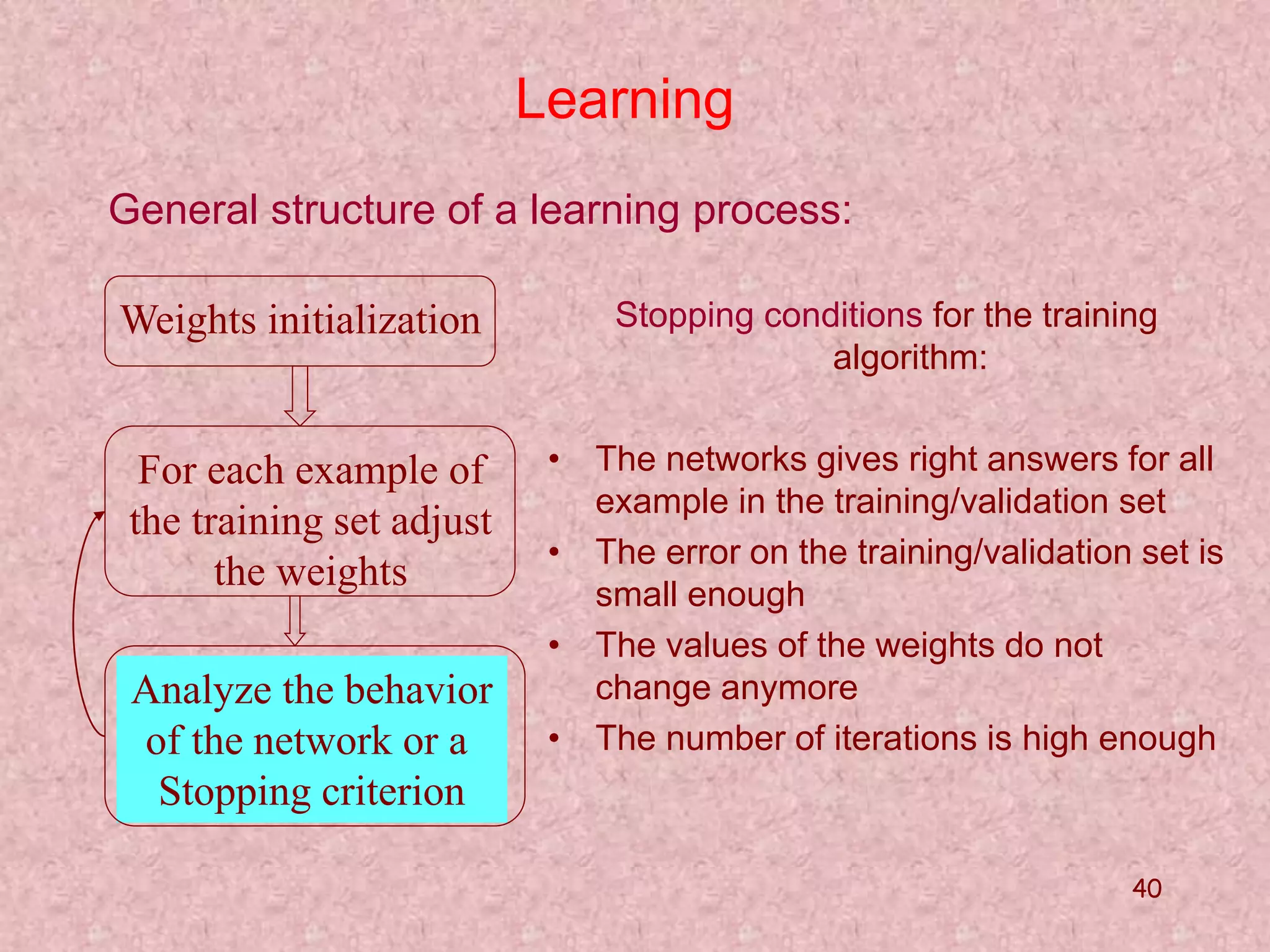
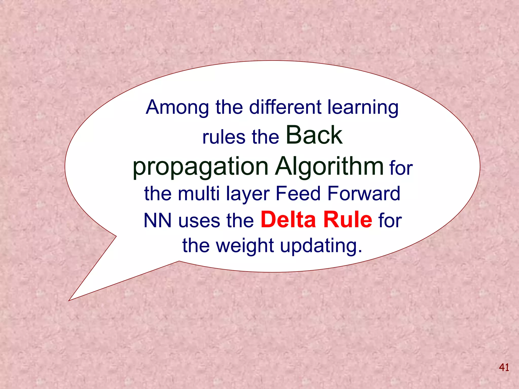
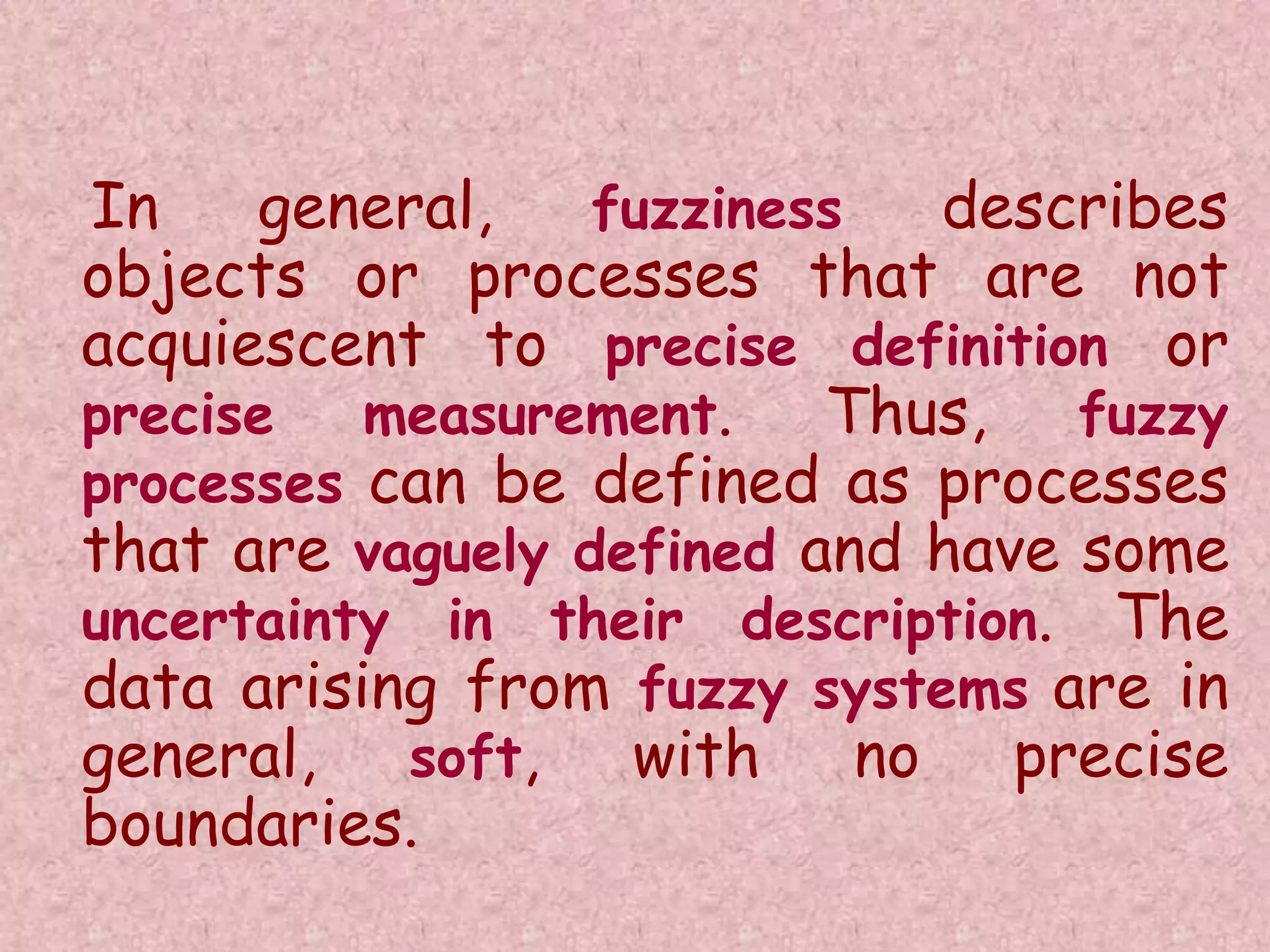
The document discusses soft computing and its techniques, including artificial neural networks (ANN). It provides an overview of ANN, including how biological neurons inspired the basic ANN model. A neuron has inputs, outputs, weights, and an activation function. Networks can be single or multilayer. Learning involves updating weights to minimize error, with backpropagation commonly used for multilayer networks. Applications include pattern recognition, function approximation, and parameter estimation. A simple example is provided to estimate the slope and intercept of a line using ANN.


![[IJET V2I2P20] Authors: Dr. Sanjeev S Sannakki, Ms.Anjanabhargavi A Kulkarni](https://cdn.slidesharecdn.com/ss_thumbnails/ijet-v2i2p20-160609043318-thumbnail.jpg?width=640&height=640&fit=bounds)


