Download to read offline
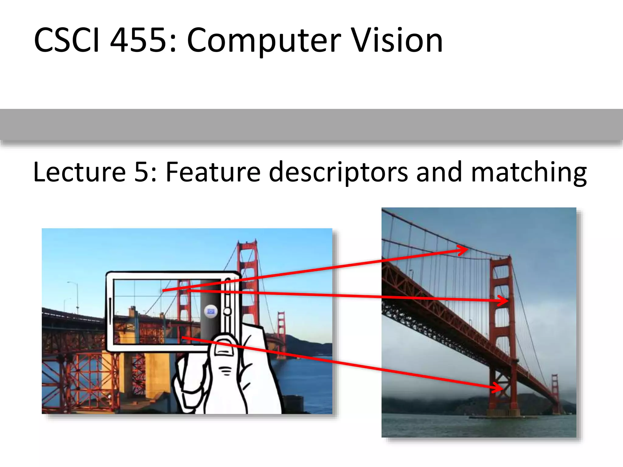

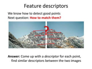
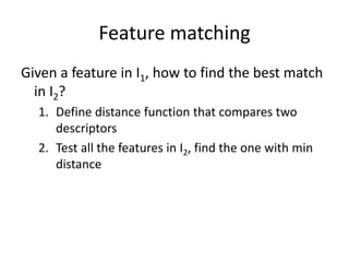
![Local features: main components
1) Detection: Identify the
interest points
2) Description: Extract vector
feature descriptor surrounding
each interest point.
3) Matching: Determine
correspondence between
descriptors in two views
],,[ )1()1(
11 dxx x
],,[ )2()2(
12 dxx x
Kristen Grauman](https://image.slidesharecdn.com/lec06descriptors-200719135145/85/Computer-Vision-descriptors-3-320.jpg)
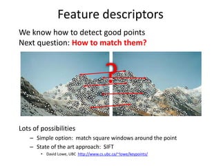

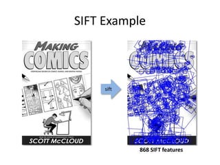

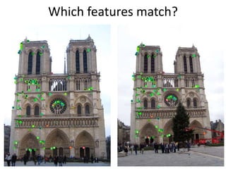
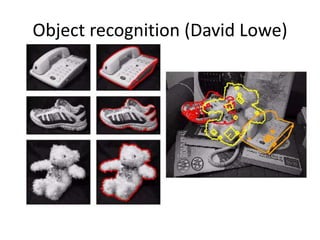
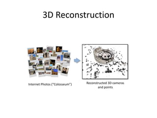


This document discusses feature descriptors and matching in computer vision. It covers three main components: 1) detecting interest points in images, 2) extracting feature descriptors around each interest point, and 3) determining correspondences between descriptors to match features across images. The document focuses on SIFT (Scale Invariant Feature Transform) descriptors, which are histograms of gradient orientations computed over localized patches that provide robust matching across changes in scale, rotation and illumination. SIFT descriptors have been widely and successfully used for applications like image stitching, 3D reconstruction, object recognition and augmented reality.


![Computer Vision - Unit-II [Repaired].pptx](https://cdn.slidesharecdn.com/ss_thumbnails/computervision-unit-iirepaired-251223052721-8dd262a0-thumbnail.jpg?width=640&height=640&fit=bounds)