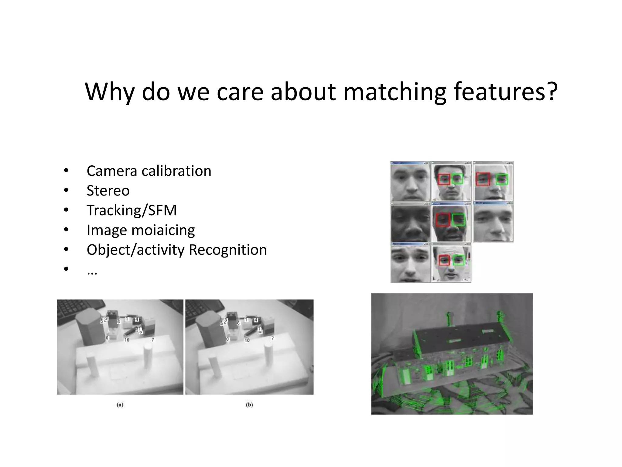
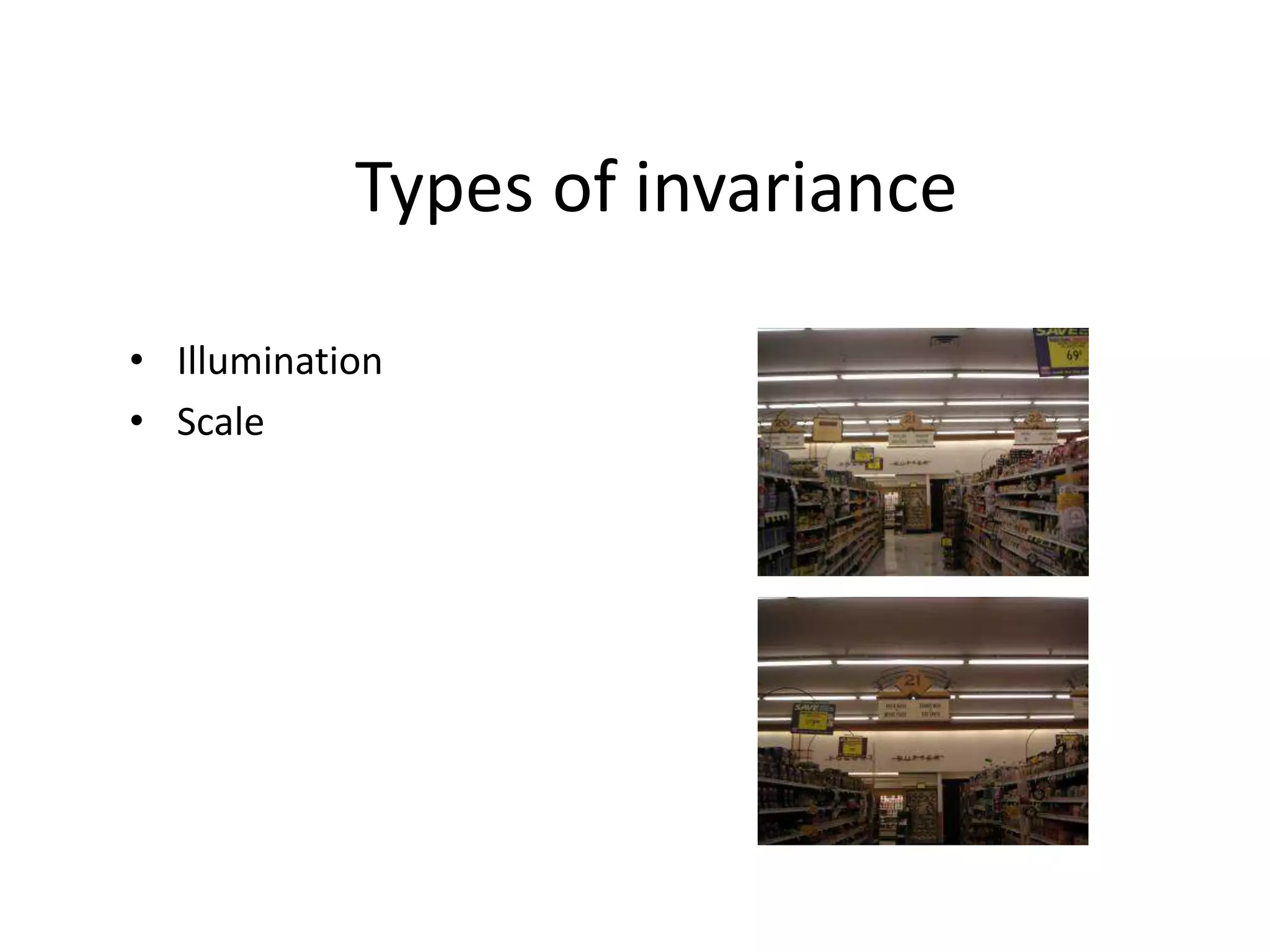
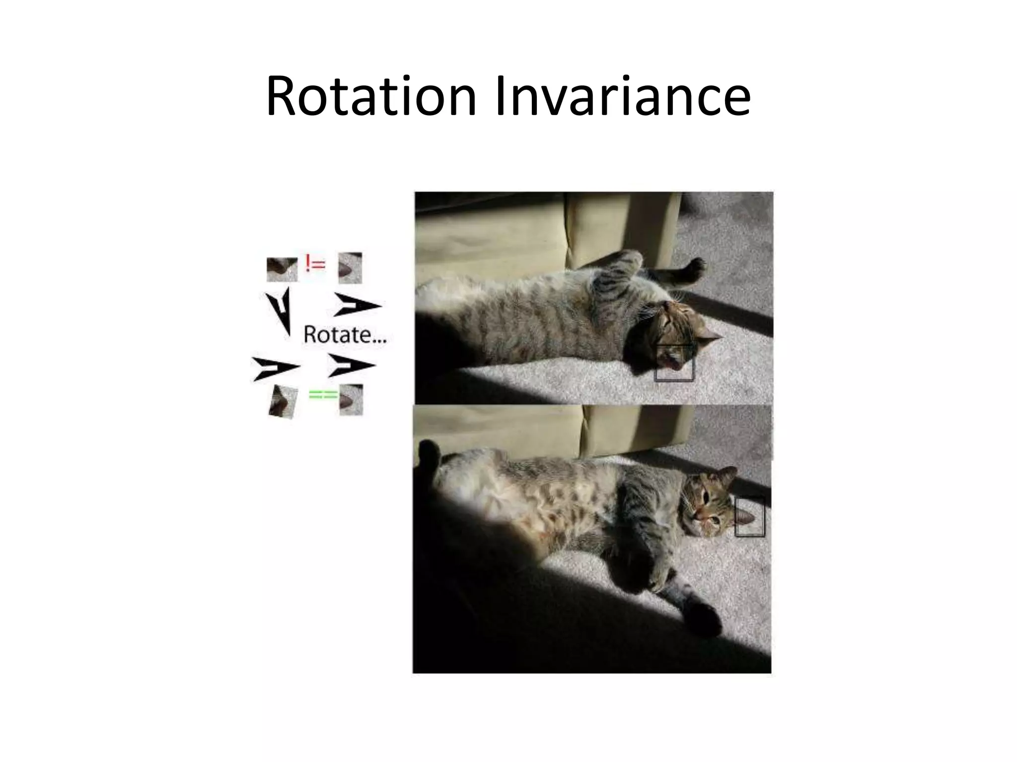
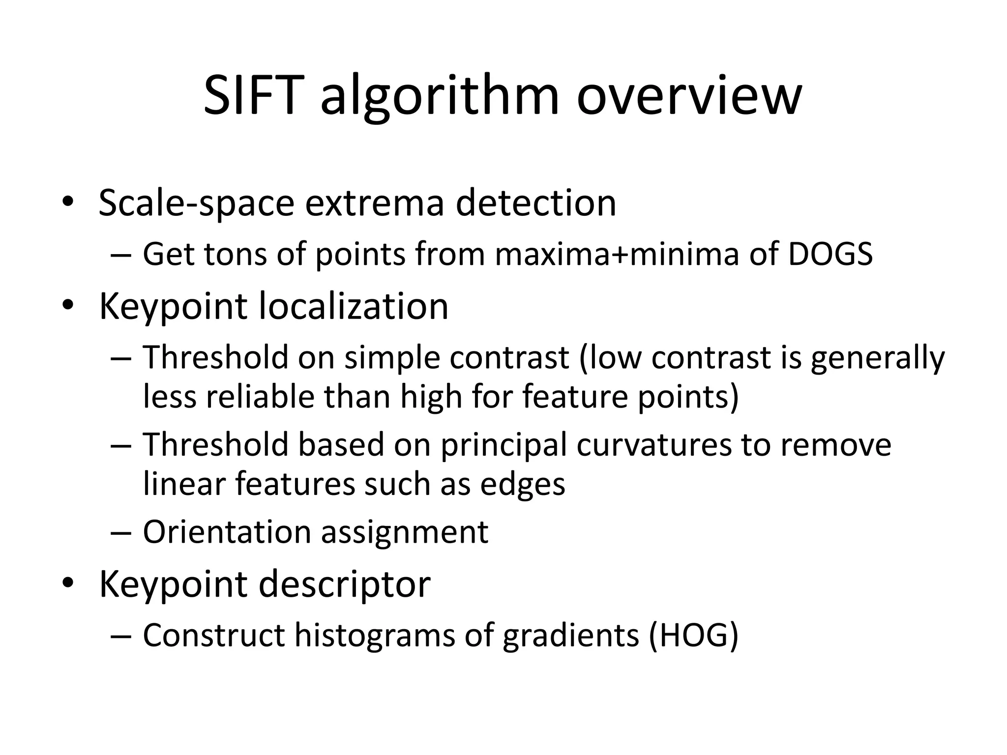
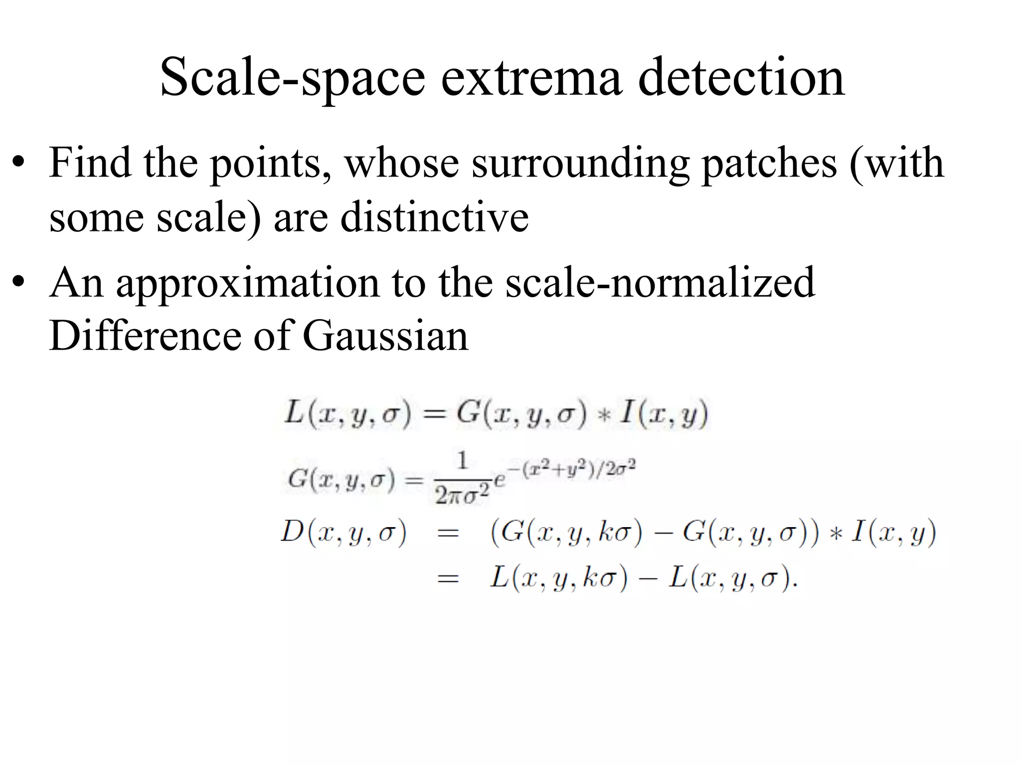
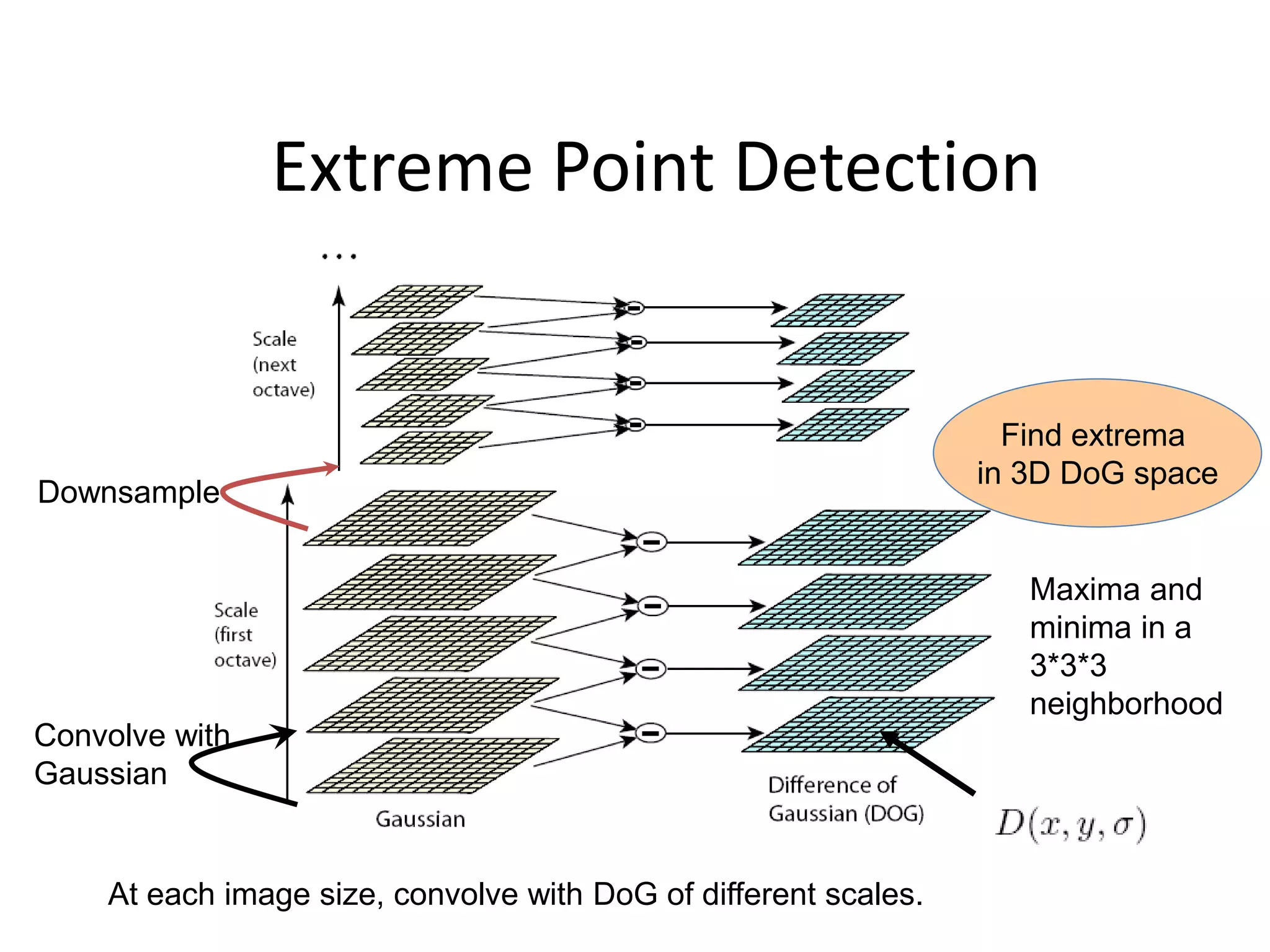
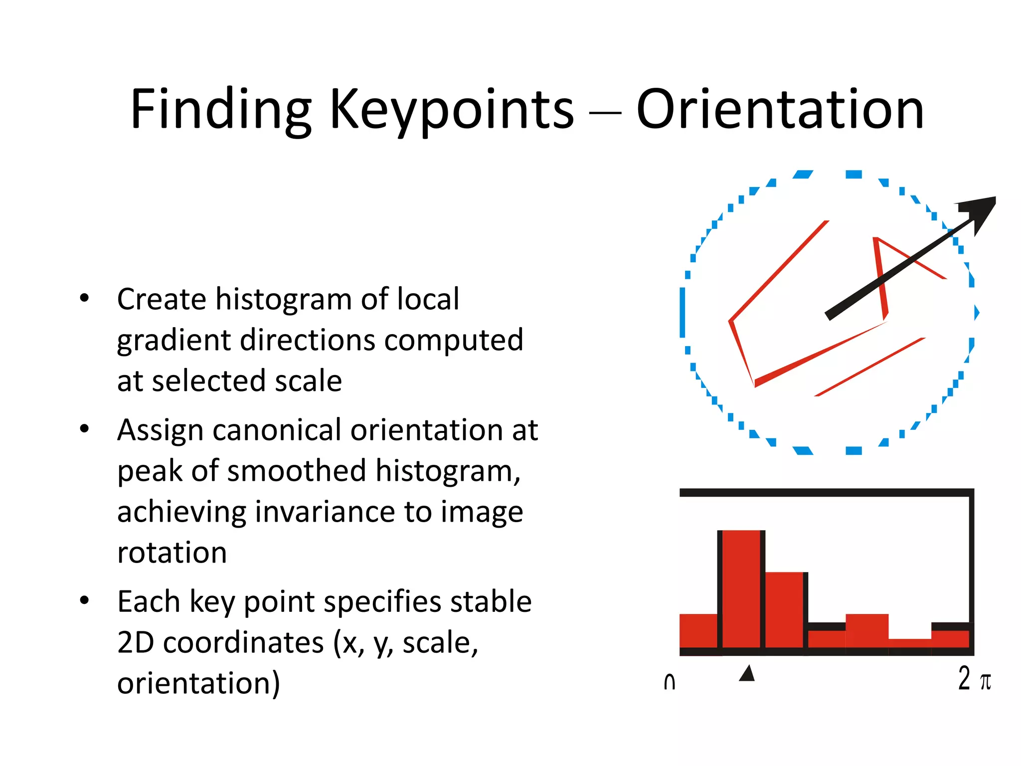
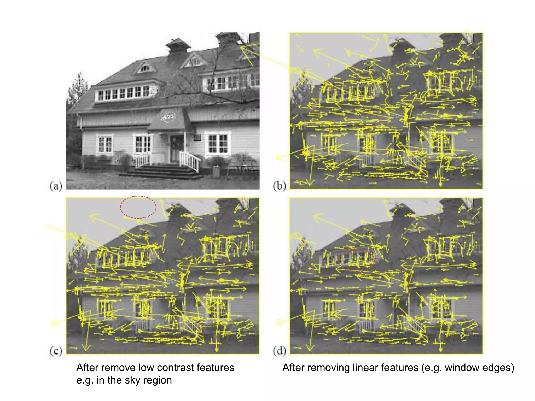
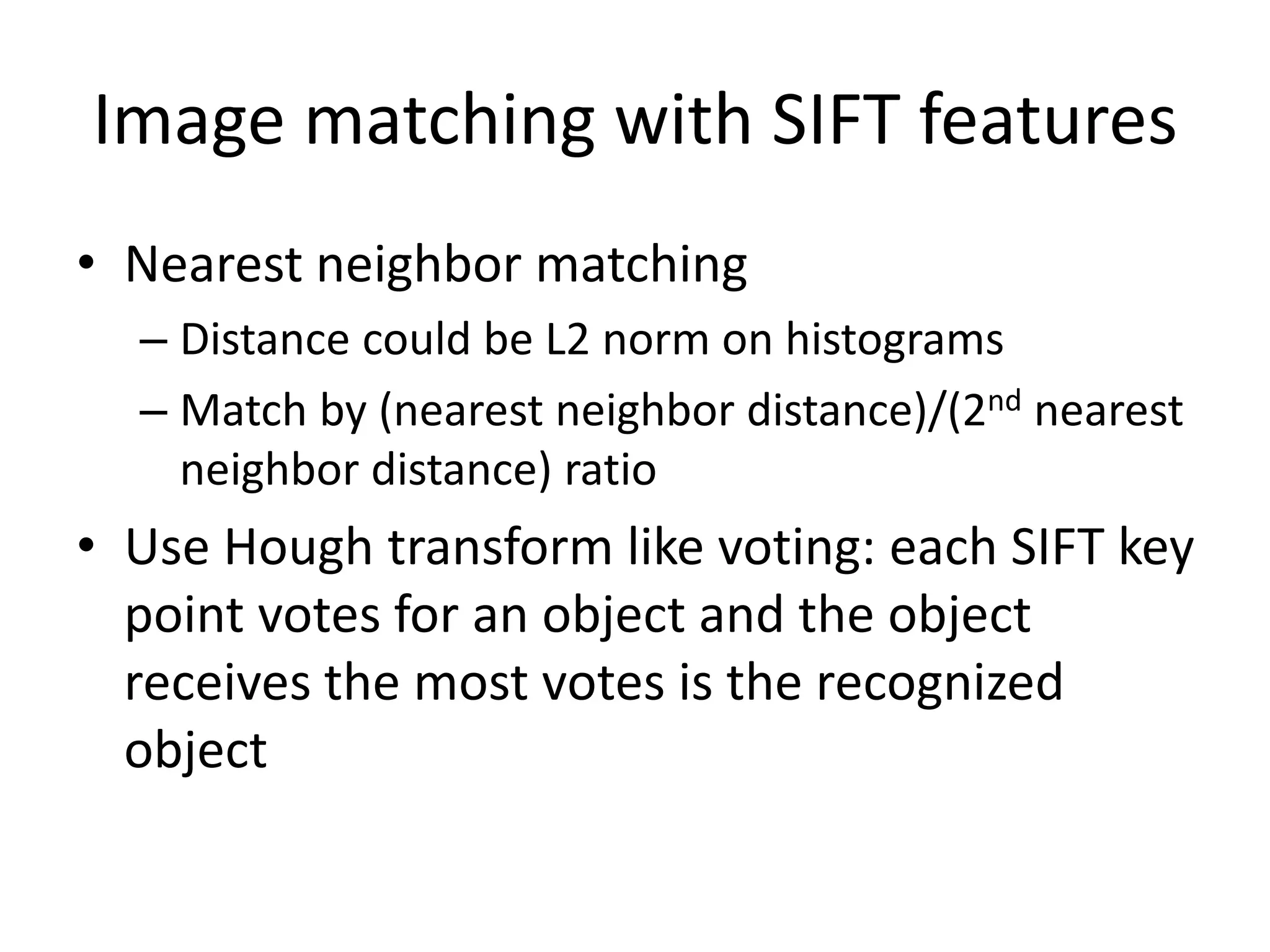
Scale Invariant Feature Transform
(SIFT)
Why do we care about matching features?
• Camera calibration
• Stereo
• Tracking/SFM
• Image moiaicing
• Object/activity Recognition
• …
Objection representation and recognition
• Image content is transformed into local feature
coordinates that are invariant to translation, rotation,
scale, and other imaging parameters
• Automatic Mosaicing
• http://www.cs.ubc.ca/~mbrown/autostitch/autostitch.html
We want invariance!!!
• To illumination
• To scale
• To rotation
• To affine
• To perspective projection
Types of invariance
• Illumination
Types of invariance
• Illumination
• Scale
Types of invariance
• Illumination
• Scale
• Rotation
Types of invariance
• Illumination
• Scale
• Rotation
• Affine (view point
change)
Types of invariance
• Illumination
• Scale
• Rotation
• Affine
• Full Perspective
How to achieve illumination invariance
• The easy way
(normalized)
• Difference based metrics
(random tree, Haar, and
sift, gradient)
How to achieve scale invariance
• Pyramids
• Scale Space (DOG method)
Pyramids
– Divide width and height by 2
– Take average of 4 pixels for
each pixel (or Gaussian blur
with different s)
– Repeat until image is tiny
– Run filter over each size
image and hope its robust
How to achieve scale invariance
• Scale Space: Difference of Gaussian (DOG)
– Take DOG features from differences of these
images-producing the gradient image at different
scales.
– If the feature is repeatedly present in between
Difference of Gaussians, it is Scale Invariant and
should be kept.
Differences Of Gaussians
Rotation Invariance
• Compute histogram of gradient directions to
identify the most dominant direction. Rotate
image to the most dominant direction.
• Rotate all features to go the same way in a
determined manner
Rotation Invariance
SIFT algorithm overview
• Scale-space extrema detection
– Get tons of points from maxima+minima of DOGS
• Keypoint localization
– Threshold on simple contrast (low contrast is generally
less reliable than high for feature points)
– Threshold based on principal curvatures to remove
linear features such as edges
– Orientation assignment
• Keypoint descriptor
– Construct histograms of gradients (HOG)
Scale-space extrema detection
• Find the points, whose surrounding patches (with
some scale) are distinctive
• An approximation to the scale-normalized
Difference of Gaussian
Extreme Point Detection
Convolve with
Gaussian
Downsample
Find extrema
in 3D DoG space
Maxima and
minima in a
3*3*3
neighborhood
At each image size, convolve with DoG of different scales.
Keypoint localization
• Eliminating extreme points with low
contrast
• Eliminating edge points
– Similar to Harris corner detector
Eliminating edge points
• Such a point has large principal curvature across
the edge but a small one in the perpendicular
direction
• The principal curvatures can be calculated from a
Hessian function or covariance matrix of gradient
(Harris detector)
• The eigenvalues of H or C are proportional to the
principal curvatures, so two eigenvalues shouldn’t
differ too much.
Finding Keypoints – Orientation
• Create histogram of local
gradient directions computed
at selected scale
• Assign canonical orientation at
peak of smoothed histogram,
achieving invariance to image
rotation
• Each key point specifies stable
2D coordinates (x, y, scale,
orientation) 0 2 
SIFT Key Feature descriptor
Take a 16x16 window of "in-between" pixels around the
key point. Split that window into sixteen 4x4 windows.
From each 4x4 window, generate a histogram of 8 bins,
producing a total of 4x4x8=128 feature vector.
SIFT Key Feature descriptor
Create the features for each SIFT key point. Given 8
orientations and 4x4 histograms, each SIFT key is described
by a vector of 128 (8x4x4) as shown below.
4 histograms with 8 direction bins
for each histogram, producing 4x8 features.
Actual SIFT stage output
After remove low contrast features After removing linear features (e.g. window edges)
e.g. in the sky region
Image matching with SIFT features
• Nearest neighbor matching
– Distance could be L2 norm on histograms
– Match by (nearest neighbor distance)/(2nd nearest
neighbor distance) ratio
• Use Hough transform like voting: each SIFT key
point votes for an object and the object
receives the most votes is the recognized
object
Application: object recognition
• The SIFT key features of training images are
extracted and stored
• For a query image
1. Extract SIFT key points and their features
2. Nearest neighbor matching or HT voting
Conclusion
• A novel method for detecting interest points.
The most successful feature in computer
vision
• Histogram of Oriented Gradients are
becoming more popular
• SIFT may not be optimal for general object
classification

SIFT.ppt

  • 1.
    Scale Invariant FeatureTransform (SIFT)
  • 2.
    Why do wecare about matching features? • Camera calibration • Stereo • Tracking/SFM • Image moiaicing • Object/activity Recognition • …
  • 3.
    Objection representation andrecognition • Image content is transformed into local feature coordinates that are invariant to translation, rotation, scale, and other imaging parameters
  • 4.
    • Automatic Mosaicing •http://www.cs.ubc.ca/~mbrown/autostitch/autostitch.html
  • 5.
    We want invariance!!! •To illumination • To scale • To rotation • To affine • To perspective projection
  • 6.
  • 7.
    Types of invariance •Illumination • Scale
  • 8.
    Types of invariance •Illumination • Scale • Rotation
  • 9.
    Types of invariance •Illumination • Scale • Rotation • Affine (view point change)
  • 10.
    Types of invariance •Illumination • Scale • Rotation • Affine • Full Perspective
  • 11.
    How to achieveillumination invariance • The easy way (normalized) • Difference based metrics (random tree, Haar, and sift, gradient)
  • 12.
    How to achievescale invariance • Pyramids • Scale Space (DOG method)
  • 13.
    Pyramids – Divide widthand height by 2 – Take average of 4 pixels for each pixel (or Gaussian blur with different s) – Repeat until image is tiny – Run filter over each size image and hope its robust
  • 14.
    How to achievescale invariance • Scale Space: Difference of Gaussian (DOG) – Take DOG features from differences of these images-producing the gradient image at different scales. – If the feature is repeatedly present in between Difference of Gaussians, it is Scale Invariant and should be kept.
  • 15.
  • 16.
    Rotation Invariance • Computehistogram of gradient directions to identify the most dominant direction. Rotate image to the most dominant direction. • Rotate all features to go the same way in a determined manner
  • 17.
  • 18.
    SIFT algorithm overview •Scale-space extrema detection – Get tons of points from maxima+minima of DOGS • Keypoint localization – Threshold on simple contrast (low contrast is generally less reliable than high for feature points) – Threshold based on principal curvatures to remove linear features such as edges – Orientation assignment • Keypoint descriptor – Construct histograms of gradients (HOG)
  • 19.
    Scale-space extrema detection •Find the points, whose surrounding patches (with some scale) are distinctive • An approximation to the scale-normalized Difference of Gaussian
  • 20.
    Extreme Point Detection Convolvewith Gaussian Downsample Find extrema in 3D DoG space Maxima and minima in a 3*3*3 neighborhood At each image size, convolve with DoG of different scales.
  • 21.
    Keypoint localization • Eliminatingextreme points with low contrast • Eliminating edge points – Similar to Harris corner detector
  • 22.
    Eliminating edge points •Such a point has large principal curvature across the edge but a small one in the perpendicular direction • The principal curvatures can be calculated from a Hessian function or covariance matrix of gradient (Harris detector) • The eigenvalues of H or C are proportional to the principal curvatures, so two eigenvalues shouldn’t differ too much.
  • 23.
    Finding Keypoints –Orientation • Create histogram of local gradient directions computed at selected scale • Assign canonical orientation at peak of smoothed histogram, achieving invariance to image rotation • Each key point specifies stable 2D coordinates (x, y, scale, orientation) 0 2 
  • 24.
    SIFT Key Featuredescriptor Take a 16x16 window of "in-between" pixels around the key point. Split that window into sixteen 4x4 windows. From each 4x4 window, generate a histogram of 8 bins, producing a total of 4x4x8=128 feature vector.
  • 25.
    SIFT Key Featuredescriptor Create the features for each SIFT key point. Given 8 orientations and 4x4 histograms, each SIFT key is described by a vector of 128 (8x4x4) as shown below. 4 histograms with 8 direction bins for each histogram, producing 4x8 features.
  • 26.
  • 27.
    After remove lowcontrast features After removing linear features (e.g. window edges) e.g. in the sky region
  • 28.
    Image matching withSIFT features • Nearest neighbor matching – Distance could be L2 norm on histograms – Match by (nearest neighbor distance)/(2nd nearest neighbor distance) ratio • Use Hough transform like voting: each SIFT key point votes for an object and the object receives the most votes is the recognized object
  • 29.
    Application: object recognition •The SIFT key features of training images are extracted and stored • For a query image 1. Extract SIFT key points and their features 2. Nearest neighbor matching or HT voting
  • 30.
    Conclusion • A novelmethod for detecting interest points. The most successful feature in computer vision • Histogram of Oriented Gradients are becoming more popular • SIFT may not be optimal for general object classification