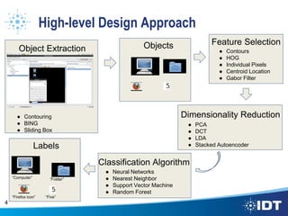
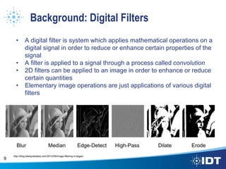
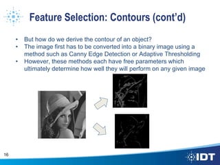
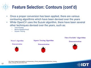
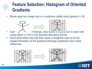
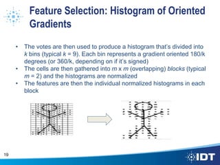
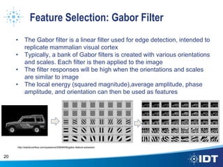
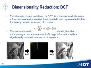
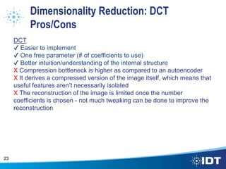
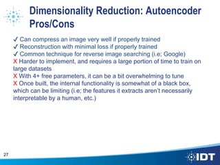
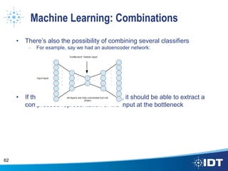
The document proposes improving object detection and recognition capabilities. It discusses challenges with current methods like different object sizes and color variations. The objectives are to build a module that can learn and detect objects without a sliding box or datastore. A high-level design approach is outlined using techniques like contouring, BING, sliding box, and feature selection methods. The design considers optimal feature selection, dimensionality reduction, and classification algorithms to function in real-time.

1. Improving Test Manager Object Detection and
Recognition
Daniel Cahall
1

2. Problem Statement
● There are a vast amount of visual objects on a screen:
o Buttons
o Symbols
o Numbers and Letters
● The current method of visual object detection and recognition is
done by scanning the screen, and looking for known images from a
datastore
● However, this is not a robust solution for this problem.
o Different object sizes
o Color variations
o Antialiasing
2

3. Objectives
• Build a module which can both learn what objects are on the
screen and detect them
• Eliminate the sliding box and datastore
3

4. High-level Design Approach
4
● Contouring
● BING
● Sliding Box
Object Extraction Objects Feature Selection
● Contours
● HOG
● Individual Pixels
● Centroid Location
● Gabor Filter
Dimensionality Reduction
● PCA
● DCT
● LDA
● Stacked Autoencoder
Classification Algorithm
● Neural Networks
● Nearest Neighbor
● Support Vector Machine
● Random Forest
Labels
“Computer” “Folder”
“Firefox icon” “Five”

5. 55
Firefox icon: 84.4% Folder: 73%
Computer: 62.4%

6. Design Overview
• Given the current state of computer vision and machine learning,
we wanted to investigate potential alternatives to the current
system.
• Identify a minimum set of features which can accurately represent
all types of visual objects, and represent them numerically
• Label each type of visual object described by the set of features
• Train a machine learning classifier on the set of features and labels
such that, when presented with an object (or any variation of the
object), it can correctly identify what the object is
• Integrate that classifier with the currently existing Testing Manager
system
6

7. Design Considerations
• What is the optimal set of features to use for classification?
• What algorithms will work effectively for:
– feature extraction
– dimensionality reduction
– classification?
• Does the final solution function in approximately real-time?
7

8. Background: Digital Signals
• A signal is a quantity which varies with respect to some
independent variable (i.e; time, space)
• A digital signal is a signal which is sampled and quantized (both the
independent variable and the quantity take on discrete values)
• An image is an example of a two-dimensional signal. In this case,
the independent quantity is space, and the dependent quantity is
color *
*in a grayscale image, it would brightness
8
http://www.solutions4u-
asia.com/emailc/digitalimageprocessing.html

9. Background: Digital Filters
• A digital filter is system which applies mathematical operations on a
digital signal in order to reduce or enhance certain properties of the
signal
• A filter is applied to a signal through a process called convolution
• 2D filters can be applied to an image in order to enhance or reduce
certain quantities
• Elementary image operations are just applications of various digital
filters
9
http://blog.teledynedalsa.com/2012/05/image-filtering-in-fpgas/

10. Feature Selection: Preprocessing
• Suppose we have a screen that looks like the one below:
• What are some of the challenges here?
10

11. Feature Selection: Preprocessing(cont)
• Some features are contingent on the size of the object - this is
bad:
– Direct pixels
– HOG
– Contours
• In order to properly correctly apply a classification algorithm, each
object has to have the same number of features
• To ensure that this does not become an issue, objects can be
normalized to one common scale before the feature selection
process.
• Okay, so the size issue has been resolved...what about the colors?
Can we normalize them too?
11

12. Feature Selection: Preprocessing(cont)
• Short answer: Yes!
• Long answer: Yes, but that doesn’t necessarily solve our problem.
• By converting a colored, 3 channel image to grayscale, all values
are normalized to a 1 channel image which ranges from 0-255.
• This results in a loss of information, which could potentially be
harmful
12

13. Feature Selection: Preprocessing(cont)
• Alternatively, 3 channels of the image can be decomposed into
their individual channels - RGB or HSV
• These single channel images can then be processed separately,
which ensures information isn’t lost
• However, some images don’t have useful information in each
channel
13
www.medialooks.com
www.wintopo.com

14. Feature Selection: Individual Pixels
• Imagine if we had a n x n pixel object, such as the 20 x 20 number
“zero” seen below:
• If we were to reduced that object to a single dimension, it would be
a 1 x n2 vector:
• We can then label that vector “zero”
14

15. Feature Selection: Contours
• Suppose we had an n x n pixel object on a screen, such as the
letter A seen below.
• We could take the outline of that object, normalize it to a common
size and location:
• and then compress it into a vector, similar to what we did before:
15

16. Feature Selection: Contours (cont’d)
• But how do we derive the contour of an object?
• The image first has to be converted into a binary image using a
method such as Canny Edge Detection or Adaptive Thresholding
• However, these methods each have free parameters which
ultimately determine how well they will perform on any given image
16

17. Feature Selection: Contours (cont’d)
• Once a proper conversion has been applied, there are various
contouring algorithms which have been devised over the years
• While OpenCV uses the Suzuki algorithm, there have been several
other techniques devised over the years, such as:
– Theo-Pavlidis
– Moore Neighborhood
– Square Tracing
17
http://www.imageprocessingplace.com/downloads_V3/root_downloads/tutorials/contour_tracing_
Abeer_George_Ghuneim/index.html

18. Feature Selection: Histogram of Oriented
Gradients
• Break apart an image into n x n patches called cells (typical n = 8)
• Compute the rate of change, also called the gradient, in each cell
using either a 1-D or 2-D discrete derivative kernel
• Each pixel within the cell then casts a weighted vote as to the
angle/orientation of the gradient (stronger gradients have more
influence)
18

19. Feature Selection: Histogram of Oriented
Gradients
• The votes are then used to produce a histogram that’s divided into
k bins (typical k = 9). Each bin represents a gradient oriented 180/k
degrees (or 360/k, depending on if it’s signed)
• The cells are then gathered into m x m (overlapping) blocks (typical
m = 2) and the histograms are normalized
• The features are then the individual normalized histograms in each
block
19

20. Feature Selection: Gabor Filter
• The Gabor filter is a linear filter used for edge detection, intended to
replicate mammalian visual cortex
• Typically, a bank of Gabor filters is created with various orientations
and scales. Each filter is then applied to the image
• The filter responses will be high when the orientations and scales
are similar to image
• The local energy (squared magnitude),average amplitude, phase
amplitude, and orientation can then be used as features
20
http://stackoverflow.com/questions/20608458/gabor-feature-extraction

21. Feature Selection: Design Decision
• Ultimately, we decided to use contours to find separate objects on
the screen, due to the domain of our problem
• Once those contours were found, the bounding box around each
contour was extracted, and the sub-image within the box was used
• In that way, we used the entire image, but contouring was
necessary for the process
• Possible future expansion: using HoG/Gabor Filter bank to locate
objects rather than contours
21

22. Dimensionality Reduction: DCT
• The discrete cosine transform, or DCT, is a transform which maps
a function in one domain (i.e; time, spatial), and represents it in the
frequency domain as a sum of cosines
• The correlated/redundant information is reduced, thereby
maintaining a maximum amount of image information with a
significantly reduced number of dimensions.
22

23. Dimensionality Reduction: DCT
Pros/Cons
DCT
✔ Easier to implement
✔ One free parameter (# of coefficients to use)
✔ Better intuition/understanding of the internal structure
X Compression bottleneck is higher as compared to an autoencoder
X It derives a compressed version of the image itself, which means that
useful features aren’t necessarily isolated
X The reconstruction of the image is limited once the number
coefficients is chosen - not much tweaking can be done to improve the
reconstruction
23

24. Dimensionality Reduction: PCA
• Principal Component Analysis is technique used to transform a set of
observations with n possibly related features into m linearly uncorrelated
features called principal components (m <= n)
• Derives a new n-dimensional coordinate system where each axis is a
principal component, and by removing the axes with least variance, maps
data points from n-dimensional space to m-dimensional space, retaining
the m features with the highest variance in the dataset
24
http://setosa.io/ev/principal-component-analysis/

25. Dimensionality Reduction: PCA
Pros/Cons
✔ Will behave similarly to an autoencoder with a single hidden layer
and an identity activation function
✔ Applied a large set of generic image tiles, PCA approximates the
DCT
✔ One free parameter (# of principal components to use)
X It’s limited in how well it can reduce the image given the complex
relationships between pixels (Restricted to linear mapping)
X Sensitive to scaling
X Makes no assumptions about the data, and so it does not optimize
for class separability*
*LDA addresses this issue
25

26. Dimensionality Reduction: Autoencoder
• An autoencoder is an artificial neural network which encodes input
data to fit in a smaller representation in the hidden layers
• It’s essentially forcing the neural network to learn how to represent
and recover data in a more compact form.
• Data provided to the neural network can be represented in smaller
and smaller forms as long as each individual layer is trained well
• Forced to learn a smaller set of useful features, rather than
compress all features
26
http://nghiaho.com/?p=1765

27. Dimensionality Reduction: Autoencoder
Pros/Cons
✔ Can compress an image very well if properly trained
✔ Reconstruction with minimal loss if properly trained
✔ Common technique for reverse image searching (i.e; Google)
X Harder to implement, and requires a large portion of time to train on
large datasets
X With 4+ free parameters, it can be a bit overwhelming to tune
X Once built, the internal functionality is somewhat of a black box,
which can be limiting (i.e; the features it extracts aren’t necessarily
interpretable by a human, etc.)
27

28. Design Decisions: Dimensionality
Reduction
• Overall, while it was investigated, the design did not require
dimensionality reduction
• However, each method was tested, and the compressed features
which the autoencoder could extract could potentially be useful for
design expansion
• Notable mention: DCT could achieve reasonable compression and
was computationally cheap relative to PCA and Autoencoders
28

29. Machine Learning: Overview
• Machine learning is the subfield of CS and ECE that’s dedicated to
giving computers the ability to learn on their own without being
explicitly programmed
• It’s applied to classification problems (i.e; identifying if a tumor is
benign or deadly), and regression (i.e; fitting a line to data points)
• In classification, data is provided in the form of a vector (called a
feature vector), along with corresponding labels.
• The machine learning algorithm will then try to derive a mapping
between the input data and the labels such that, when fed new
data, it will provide the correct label.
• While each algorithm derives the relationship differently, they’re all
just trying to solve an optimization problem
29

30. Machine Learning: Optimization
• The objective of each algorithm is to map a relationship between
the data, the inputs, and labels, the outputs, with minimal error
• We’re trying to find the global minimum of the error function, which
is the a function of the difference between the expected outputs
and the predicted outputs
30
http://alykhantejani.github.io/images/gradient_desc
ent_line_graph.gif
http://mccormickml.com/2014/03/04/gradien
t-descent-derivation/

31. Machine Learning: Precautions
• Overfitting: The model learns the noise in the training data rather than the
underlying relationship, and so it does not perform well when provided new
validation data.
• Curse of dimensionality: With a finite amount of training data, the spread of
the data becomes sparser as dimensionality increases. Furthermore, more
features are more computationally expensive.
• Underfitting: The model hasn’t learned enough about the data to make
accurate predictions on the validation data
• Class imbalances: During training, if there are significantly more samples
in one class then another, this could affect how the model learns
31 http://scikit-
learn.org/stable/auto_examples/model_selection/plot_underfi
tting_overfitting.html

32. Machine Learning: Bias vs. Variance
• In more technical terms, straddling between overfitting and
underfitting is called the bias-variance tradeoff
• Bias is a measurement of how far off predictions are from the
correct value on the training data
• Variance is a measurement of variability in the predictions on the
training data, regardless of correctness
• A model with high bias will tend to underfit the data
• A model with high variance will tend to overfit the data
• Ideally, our model will have low bias and low variance
• Simplicity vs. Predictive Ability
32 http://scott.fortmann-roe.com/docs/BiasVariance.html

33. Machine Learning: Hyperparameters
• A hyperparameter is a variable which defines high-level concepts
about an algorithm, such as its complexity or learning capacity
• In any given ML algorithm, there are one or more hyperparameters
which determine how well it will perform (regression or
classification) on any given dataset
• There are then a set (or several sets) of hyperparameters which will
provide the best classification/regression performance
• Oftentimes, they are arbitrarily chosen from a “suggested range” by
the engineer or scientist analyzing the dataset. In that way, they are
just tuning knobs.
33

34. Machine Learning: Hyperparameter
Optimization
• Grid search - If you have n hyperparameters, an n dimensional grid
is created based on a range of values for each parameter. From
there, it is a brute force search (although easily parallelizable)
• Random search - Creating an n-dimensional grid, and randomly
sample from it. Surprisingly effective, and less computationally
expensive than grid search
• Gradient optimization - Essentially performing gradient descent on
the hyperparameters
34 http://www.jmlr.org/papers/volume13/bergstra12a/bergstra12a.pdf

35. Machine Learning Algorithms: SVM/SVC
• Suppose we have an n-dimensional dataset which is linearly
separable
• In this feature space, there are many n-1 dimensional planes which
provides separation between the classes
• A support vector machine is a classifier which, given a labeled
dataset, will derive a hyperplane (or set of hyperplanes) which
optimizes for maximum class separability
35
docs.opencv.org

36. Machine Learning Algorithms: SVM
(cont’d)
• However, what if our data looked like this:
• Uh oh. It isn’t linearly separable in n. If we tried to derive a
separating line in n, it would perform very poorly.
36 http://www.eric-kim.net/eric-kim-net/posts/1/kernel_trick.html

37. Machine Learning Algorithms: SVMs
(cont’d)
• Does this mean that an SVM is only limited to linearly separable
data in n?
• Short answer: Yes…
• Long answer: Yes, but what if we could toy with n?
• Let’s look at that example again, but project it to 3D:
• It’s separable in n+1!
37
http://www.eric-kim.net/eric-kim-net/posts/1/kernel_trick.html

38. Machine Learning Algorithms: SVMs
(cont’d)
• We can therefore derive a linear separation in m-dimensional space (m>n), and then
project that separation back down to n-dimensional space - even if the separation
in n no longer necessarily linear
• A function called a kernel function, usually denoted by ɸ, when applied to a set of n-
dimensional vectors, implicitly computes the dot product in m-dimensional space
(m>n)
• This is called the kernel trick, and it enables us to determine the non-linear decision
boundaries without explicitly projecting our data into higher dimensional space
38
http://www.eric-kim.net/eric-kim-net/posts/1/kernel_trick.html

39. SVM Pros & Cons
✔ Not many hyperparameters (typically 2: C and Gamma)
✔ Global optimum is guaranteed (convex optimization)
✔ It can be argued that the math and intuition behind SVMs can be
derived and understood pretty easily
✔ Not prone to overfitting
X Kernel needs to be guessed (although RBF is typically a good
assumption)
X Non-parametric (complexity grows with the number of training
samples)
39

40. Machine Learning Algorithms: kNN
• In n-dimensional feature space, there are several clusters which
correspond with the different classes
• In k-Nearest Neighbor, a new point is placed in the feature space, and
classified based on what classes the k closest points are
• Usually k is an odd value, to avoid the situation of a tie between classes
• Alternatively, the decision could be made based off of a weighted distance
metric (i.e; closer points have more weight).
• One of the simplest classification algorithms, but it can be computationally
pretty heavy
40

41. Machine Learning Algorithms: kNN
(cont’d)
• Suppose there are M points in n-dimensional space
• When a new observation is provided, that will be M distance
calculations to determine the nearest neighbor, and M that need to
be stored and compared
• In Euclidean distance, that doesn’t scale well - a squared sum of n
values M times
• For this reason, there are alternative distance metrics
41
http://ocw.metu.edu.tr/pluginfile.php/4877/mod_resource/content/1/Min720lecture
notes_3.pdf

42. Machine Learning Algorithms: kNN
distance metrics
• City block distance: The sum of the absolute difference in Cartesian
coordinates
• Minkowski metric when k = 1
42

43. Machine Learning Algorithms: kNN
distance metrics (cont’d)
• Hamming distance: a similarity metric of two Strings
• The minimum number of substitutions required to convert one
string into another
• In two binary strings a and b, it would correspond to the number of
1’s in a XOR b
• Ex:
– H(“Danny”, “Manny”) = 1
– H(“01010101”, “11011110”) = 4
43
http://www.eli.sdsu.edu/courses/spring96/cs662/notes/networks/networks.html

44. Machine Learning Algorithms: kNN
distance metrics (cont’d)
• Cosine similarity + LSH:
– Produce K planes in the feature space
– Assign a value of 0/1 based on whether the new data point is
further right or left (<180 or >180 degrees) to the plane such
that you have a K length binary string
– Compute hamming distance to determine angle, and apply
cosine function
– The result will vary from 1 (identical) to -1 (opposite)
44
http://www.bogotobogo.com/Algorithms/Locality_Sensitive_Hashing_LSH_using_Cosine_Dist
ance_Similarity.php

45. Machine Learning: kNN Pros/Cons
✔ Easy to implement - no training and one parameter
✔ Intrinsically handles multi-class classification
✔ Intuitive and flexible
X Memory and time usage (scales linearly with respect to samples)
X Uses all features (doesn’t learn which ones are most important for a
decision)
X In higher dimensions, performance degrades because the
“neighborhood” gets larger. For an N sample dataset in d dimensions,
distance to the k nearest neighbors scales on average at a rate of
(k/N)1/d
45

46. Machine Learning Algorithms: Random
Forests
• A form of ensemble learning which uses N tree predictors, called a
forest (hence the name)
• Each tree in the forest selects a subset of the training data to train
on. The sampling is done with replacement, so there is potential
overlap (a training sample could be used in several trees)
– This technique is known as bootstrapping
• At each node in the tree, a random subset of the features is
selected as a splitting criterion
• Once trained in this fashion, each tree in the forest takes an
observation and classifies it. The classification with the most votes
from each tree in the forest is considered the correct label
• Can be parallelized, during training, because each tree can be
trained independently
46
http://file.scirp.org/Html/6-9101686_31887.htm

47. Machine Learning Algorithms: Random
Forests
• The bias of the overall model has the bias of a single decision tree -
which, individually, has high variance
– However, since the output is the average of each tree in the
forest, the overall variance is greatly reduced
• In the case of regression, rather than using the voting system, the
outputs of all the trees would be summed and averaged
• Random Forests are unique in that with the voting system, the
confidence in a decision can be determined
• This information can prove to be useful when analyzing the
success of the classifier
– It enables us to dissect individual instances rather than analyzing just the
overall performance
47

48. Machine Learning: Random Forest
Pros/Cons
✔ Can be parallelized (each tree in the forest can be trained
separately)
✔ Great bias-variance tradeoff
✔ Inherently does a form of cross-validation
✔ Few parameters to tune (number of trees in the forest is the most
significant one)
X If the data is too noisy or sparse, it could be prone to overfitting
X Computational complexity is linear with respect to the number of
trees (depth) in the forest. For a sufficient amount of data, training takes
some time
48

49. Machine Learning Algorithms: AdaBoost
• A weak classifier is a model which performs only slightly better than
random guessing (i.e; a decision stump)
• Suppose we had a set of N weak learners and applied them to an
M sample dataset in a sequential fashion. Each sample in the data
starts out with a weight of 1/M.
• The first learner will then train on the dataset. The samples which
are classified incorrectly most often (or considered “harder to
learn”) are penalized by increasing the weight
• Once a designated number of iterations has been reached, the
data is sent to the next classifier, which will then focus on the more
weighted samples
• The final predictions on all samples are determined using a
weighted voting system from each classifier
49

50. Machine Learning Algorithms: AdaBoost
(cont’d)
• This is a method of ensemble learning called adaptive boosting,
abbreviated AdaBoost
• Ensemble members are trained on subsets of the training data, and each
additional classifier is trained on data that are biased towards samples
which were misclassified by the previous classifier
• In this way, it focuses on increasingly difficult to learn samples
50
“They're crude and unspeakably plain...But maybe they've a glimmer
of potential, if allied to my vision and brain”

51. Machine Learning: AdaBoost Pros/Cons
✔ No prior knowledge of the weak classifiers is required
✔ Relatively easy to implement
✔ No parameters to tune (aside from number of weak classifiers)
X Sensitive to outliers
X Depending on the choice of weak classifier, overfitting could be an
issue
X Can’t be parallelized
51

52. Machine Learning: Artificial Neural
Networks
• A structure which has an input layer, N “hidden layers”, and an
output layer, where each layer consists of one or more neurons
which connect to neurons from the previous layer and the next
layer
• The output values from the neurons in one layer are
weighted,summed, and applied to each neuron in the next layer
• This weighted sum is then transformed by means of an activation
function, and output to the next layer
52
docs.opencv.org

53. Machine Learning: ANN Activation
Functions
• Activation function f(u): defines the output of a neuron based on an
input.
– The input is the weighted sum of the outputs from the neurons in the previous
layer
– Each layer can have a different activation function for its neurons
– Function must be differentiable (the rate of change can be computed)
– For non-trivial problems, the activation function is usually non-linear (i.e;
exponential, Gaussian)
53
http://stats.stackexchange.com/questions/188277/activation-function-for-first-layer-nodes-
in-an-ann

54. Machine Learning: ANN Activation
Functions (cont’d)
Sigmoid
• One of the most
commonly used
activation functions
• Large negative numbers
tend to 0, Large positive
numbers tend to 1
• However, the rate of
change drastically
decreases for extremely
large/small values - this
means the derivative is
near 0, which is
problematic for
backpropagation
54
ReLU
• Rectified Linear Unit
• Essentially computes
max(0,x), thresholding at
0
• Less computationally
expensive than sigmoid
• Doesn’t face the unstable
gradient problem
• However, output is not
constrained like the
sigmoid
Identity/Linear
• Only allows linear
transformations of data
• Behaves as single
perceptron, regardless
of the number of layers
• Extremely limited, and
not used frequently
unless in conjunction
with other, non-linear
layers
Note: Hyperbolic
tangent and leaky
ReLU are derivatives
of sigmoid and ReLU
http://cs231n.github.io/neural-networks-
1/#actfun

55. Machine Learning: ANN
Backpropagation
• The weights are then adjusted by means of a method called backpropagation,which works to
minimize the error, starting from the output layer
• After each iteration of backpropagation, the weights are adjusted by a free parameter called
learning rate and the current rate of change with respect to each weight
• This process is repeated until the error has been minimized to some desired value, or another
termination condition has been met (using gradient descent)
55
https://www.researchgate.net/figure/223521884_fig6_Fig-6-Schematic-diagram-of-back-propagation-neural-networks-with-two-hidden-layers"><img
src="https://www.researchgate.net/profile/Lucio_Soibelman/publication/223521884/figure/fig6/AS:305169624518662@1449769516864/Fig-6-Schematic-diagram-of-back-
propagation-neural-networks-with-two-hidden-layers.png" alt="Fig. 6. Schematic diagram of back-propagation neural networks with two hidden layers.

56. Machine Learning: Artificial Neural
Networks (cont)
• Free parameters:
– Learning rate
– Regularization Term
– Activation function
– Activation function parameters
– Weight decay (opt)
– Momentum (opt)
• It’s a bit overwhelming, and there is no direct way to compute the
optimal set of values - it varies by the problem. However, most
parameters have a ballpark range
• By understanding what each parameter does, tuning will usually
obtain an adequate solution, although hyperparameter optimization
techniques will (probably) find you the the optimal solution
56

57. Machine Learning: Neural Network Pros
& Cons
✔ Many variations - the number of neural network configurations could
be compared to the number of machine learning classifiers
✔ Can have multiple outputs - such as a probability distribution or a
replica of the input
✔ Current state-of-the-art - many of the big accomplishments in the ML
space in the last 5 years have been from Neural Networks
✔ Identifies useful features during training
X Many hyperparameters (e.g; learning rate) and model parameters
(e.g; number of nodes in a hidden layer, number of hidden layers)
X Functions somewhat as a “blackbox” - while we know what’s going
on, we’re not intimately familiar with it
X Requires a lot of data to perform well, and be worth the
computational expense
X Prone to overfitting
57

58. Convolutional Neural Networks (CNN)
• A convolutional neural network is a specific type of ANN which
attempts to replicate the mammalian visual cortex though the
connectivity of its neurons
• Each layer of a CNN is comprised of a collection of 2D filters,
represented by a set of neurons, which processes small portions of
an image (3x3 or 5x5). These are called the convolution layers.
• The convolution layers are followed by pooling layers, where the
outputs are fed into a filter, which processes and extracts the
designated value from small patches of the output (2x2)
• This process is repeated for the designated number of hidden units
in the network.
• The name derives from the fact that a digital signal is filtered by a
process called convolution with the impulse response of a digital
filter
58

59. CNN’s (cont’d)
• While the filters only cover a portion of the input at a time, they
always extend the volume (channels) of the image
• The number of filters used in the convolutional layer is the volume
of the output
• The size of the activation is contingent on the filter size and the
stride size
• Max pooling is the typical downsampling method, but there is also
average pooling and stochastic pooling
59
http://deeplearning4j.org/convolutionalnets.html

60. CNN Visuals
60
http://deeplearning4j.org/convolutionalnets.html

61. CNN Parameters
• Stride size (S) - how fast the filters and pooling layers slide across
the image.
– Typically S = 1 for a filter and S = 2 for pooling
– This ensures that spatial downsampling is primarily done by
pooling - information isn’t lost in the filtering layer
• Filter / Pooling Receptive Fields- the dimensions of your filter and
downsampling layers.
– The filter shape usually depends on the size of the image
– the pooling layer is typically 2x2. Too large and useful
information can be discarded.
• Depth (K) - the number of filters used
• Plus the original Neural Net parameters (learning rate, momentum,
etc.)
61

62. Machine Learning: Combinations
• There’s also the possibility of combining several classifiers
– For example, say we had an autoencoder network:
• If the network was trained properly, it should be able to extract a
compressed representation of the input at the bottleneck
62

63. Machine Learning: Combinations
(cont’d)
• That compressed representation could then be extracted, and fed
into another classifier or regression algorithm
• Visually, this model could be represented as follows:
• In this way, the features considered most important are used for
classification
– Dimensionality reduction is inherently part of the model
63
● SVM
● Softmax
Regression
● Random
Forest
label

64. Okay, so, knowing all of that...
64

65. Machine Learning: Design Decisions
• It’s a difficult decision, given the pros/cons of each algorithm.
• It’s not like there’s a wrong answer. Each algorithm, if tuned
properly, could probably perform the designated task at a
reasonable level of success. After all, they’re just solving an
optimization problem.
• After testing each algorithm and reviewing different sources, we
ultimately decided to use an artificial neural network
• To be specific, a convolutional neural network, or CNN.
65

66. Machine Learning: Design Justification
• While neural networks are a bit more difficult to understand and
implement, they have proven effective when tuned properly
• Furthermore, while most of the algorithms are general for datasets,
the CNN is pretty specific to image processing applications
• Neural networks inherently provide the confidence of the
classification, whereas most other algorithms don’t explicitly do
that. In this application, we’re interested in probability
• Lastly, in terms of the open problem of multi-label classification
(which is also our problem), most work on that front recently has
been done by CNNs
• That being said, future work could be expanding this design to fit
other algorithms, or even building an ensemble
66

67. Dataset Production
• Initially, data was sparse (300+ classes, 1-20 samples per class)
• In order to ensure that data sparsity wasn’t an issue, artificial
images were created using HSV channel isolation, morphological
operations, and blurring
• This produced 200+ additional images per one image.
67
. . .

68. Dataset Production (cont’d)
• Of course, there are many more variations that could be made to
produce even more data
– For a rotationally invariant classifier, rotated images could have
been used during training
– RGB channels could be isolated
– Other morphological operations (opening, closing, sharpening,
etc.)
• However, producing the data costs time
• And more data means more training, which also costs time
• Past a certain threshold, performance will be minimally improved or
even potentially degraded, for the time invested in producing and
training on more data
68

69. CNN Performance Analysis
• In order to analyze the performance of the CNN on the dataset, we made use of the
Histogram Iteration Listener which the deeplearning4java library provides
69 http://deeplearning4j.org/visualization

70. CNN Performance Analysis
70
Top Right: Error vs. Iteration
● Should be decreasing and tending towards 0
● If it’s increasing/going unstable, the learning rate
could be too high
● Oscillations could be due to low batch size
Top Left: Weights/Bias Histogram:
● Weights should appear to be a
Gaussian/normal distribution after some time
● This is because weights should be low (near 0)
and so a majority will have a magnitude around
that bin
● Biases should follow the same trend
● If extreme values are observed, there could be
issues with the learning rate, weight decay, or
momentum parameters
Bottom Right: Gradient Histogram
● Gradients should be low overtime
(weights should not be changing
drastically)
● Therefore, the distribution should
also look (approximately)
Gaussian
● If extreme values are observed,
that could be due to an unstable
gradient (exploding/vanishing)
Bottom Left: Average Weight/Bias
Magnitudes:
● Large spikes/changes could mean that
the gradient is unstable
● Should stay reasonably flat after
several fluctuations (with some degree
of noise)

71. CNN Performance Analysis
• In addition to the Histogram Listener, dl4j also provides statistics about the
classifier:
– Accuracy: TP+TN/Total
• Typical measure of correctness, and intuitively how the performance of
classifier is measured - TP+TN/(TP+FP+FN+TN)
– Precision: TP/TP+FP
• How many of the returned positives were true positives?
– Recall: TP/TP+FN
• Out of all positive cases, how many were actually classified as positive?
– F1: 2*Precison*Recall/(Precision+Recall)
• Battles the “Accuracy paradox” which can occur if there’s a large class
imbalance (i.e; a “dumb classifier” can do better than a trained one)
• Arguable a better metric of classifier performance
• In order to analyze the data even further, we also generated a confusion
matrix
– Allows us to analyze on a case by case basis
– Provides a visual for the statistics provided by the listener
71

72. Overall Design Structure
72
CNN
Firefox icon: 84.4% Folder: 73%
Computer: 62.4%
R
E
S
I
Z
E
R
Adaptive
Thresholding

73. Design Parameters
• CNN parameters:
– Filter Shape = 3x3 (both layers)
– Stride = 1 for filters, 2 for pooling
– Number of filters = 20 in first layer, 50 in second
– Learning rate = 0.015
– Momentum = 0.95
– Weight Decay = 0.0
– Number of layers = 5
– Activation Function = Sigmoid
– Image sizes = 28 x 28
• Contouring Parameters
– Binary conversion method = Adaptive Threshold
– Contour approximation method
– Parameters of conversion method
• Adaptive Threshold: Block size, offset, adaptive method,
threshold type
• Canny: Upper and lower thresholds
73

74. Design Results
• With 3 epochs:
– Accuracy: 94%
– F1 Score: 95%
– Precision: 94%
• Times:
– Total Time: 24.154 s
– Average Time: 2.7 ms
– Max Time: 26 ms
– Median Time: 2 ms
– Min Time: 1 ms
74

75. Design Advantages
• Neural networks output probabilities in order to make decisions -
which means you get the level of confidence in a decision
– Not as easily done with other classifiers
– Gives you more insight than just providing a label
• Extracts and trains on useful features during training
– As humans, there are patterns and characteristics that we can’t pick up on but
that combinations of filters will
– This removes feature selection from the design process
• Flexibility
– While the number of free parameters is a bit excessive, it also makes it an
extremely useful tool to solve a variety of problems
– Also, that means that somewhere in hyperparameter space, there is probably a
set of values which will work for all images in our dataset
75

76. Design Caveats
• Classifier complexity - while implementation isn’t too difficult,
optimization is challenging with the number of free parameters
– Furthermore, parameters which work well for one image may not achieve the
same success for another image
• Training time - training on the data takes an immensely long time,
which may not scale well.
– Parallelize when possible
• Somewhat prone to overfitting
• On a similar vein to the parameter issue, contouring algorithm
parameters which work well for one image may not transfer over
well
– Automating those parameter adjustments may be worth looking into, although
that is an open problem in computer vision
76

77. Possible
Expansion/Improvements/Alternatives
• More modularity
– make OpenCV/dl4j integrate a bit more seamlessly
– A GUI would make training a bit cleaner too
• Training on a GPU
– Faster training which would make prototyping ideas easier
– On that end, parallelization may be possible
• Combining an Autoencoder and a CNN
– I haven’t looked extensively into this - too much information may be lost in that
process. Also, improvements may be none or minimal
• Simplifying the design
– Applying a single-layer CNN is similar to applying a Gabor Filter bank
– We may be able to get away with using Gabor filters and using the responses
(power, phase, etc) as features in a simpler classifier
• Layers - the more, the better?
• Formal hyperparameter tuning
• Feature compression - LDA
– Linear Discriminant Analysis tries to maximize class separability in its
compression
77

78. And the list goes on….
• There are plenty more ML algorithms which haven’t been
mentioned in any depth here
• Furthermore, there are many variations of algorithms which haven’t
been completely investigated
– Recurrent Neural Networks
– Extremely Randomized Forest
– Gradient Boosted Forests
• This does not discount them from being a viable candidate in the
final system
78

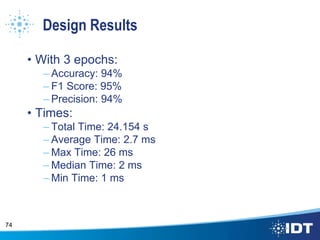
79. Typical Neural Net Parameter Values
• Learning rate
– Domain: [0, 1]
– Typical value(s): 0.01-0.2
• Momentum
– Domain:[0,1]
– Typical value(s): 0.8-0.9
• Hidden Layers
– Domain: infinity…?
– Typical Values: Between the number of output nodes and
number of input nodes
• Weight decay
– Domain: [0,1]
– Typical Values: 0.01-0.1
79