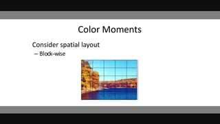
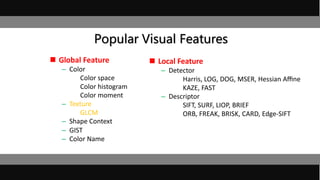
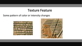
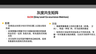
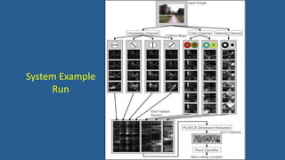
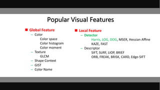
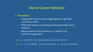
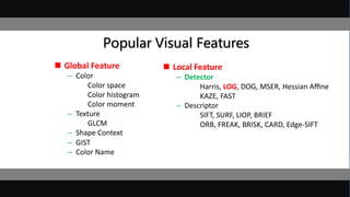
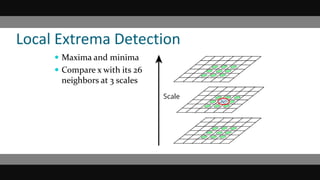
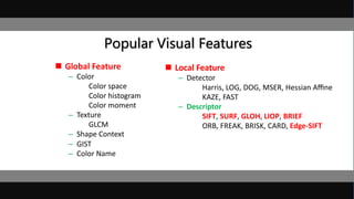
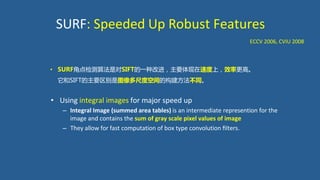
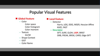
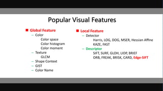
This document discusses various image features that can be used for large-scale visual search and content-based image retrieval (CBIR). It describes both high-level semantic features and low-level visual features that can be extracted from images. For low-level features, it outlines several popular global features like color histograms, color moments, texture descriptors using gray-level co-occurrence matrices (GLCM), shape context, and GIST. It also discusses commonly used local feature detectors like Harris corner detector, SIFT, and descriptors like SIFT, SURF, BRIEF.

1. Large-‐scale Visual Search:
CBIR -‐Features
Weimin Tan. Fudan University sep, 2014

2. Image features
Levelsofimagecontent
High-level features Semantics
 Shape
 Texture
 Color, lightness
Low-level features / visual features
(signatures, descriptors)

3. Image features
Textual Visual (low-‐level)
Annotations and metadata:
– tags/keywords;
– Creation date;
– geo tags;
– name of the file;
– photography conditions
(exposition, aperture, flash…).
Features extracted from pixel values:
– color descriptors;
– texture descriptors;
– shape descriptors;
– Spatial layout descriptors.

4. Visual features (Low-‐level)
Global Local
Describe the whole image:
– average intensity;
– average amount of red;
− …
Describe one part of the image:
– average intensity for the left
upper part;
– average amount of red in the
center of an image;
− …
All pixels of an image are processed. Segmentation of the image is performed, pixels of a
particular segment are processed to extract features.

5. Popular Visual Features
 Global Feature
– Color
Color space
Color histogram
Color moment
– Texture
GLCM
– Shape Context
– GIST
– Color Name
 Local Feature
– Detector
Harris, LOG, DOG, MSER, Hessian Affine
KAZE, FAST
– Descriptor
SIFT, SURF, LIOP, BRIEF
ORB, FREAK, BRISK, CARD, Edge-SIFT

6. • Quantization of color space
– Quantization is important: size of the feature vector.
– When no color similarity function used:
• Too many bins – similar colors are treated as dissimilar.
• Too little bins – dissimilar colors are treated as similar.
h1 h2 hN
Color Histogram

7. Color Histogram Retrieval

8. Color Histogram
Advantage :
• The color histogram is easy to compute and effective in characterizing
both the global and local distribution of colors in an image.
• Robust to translation and rotation about the view axis and changes
only slightly with the scale, occlusion and viewing angle.
Disadvantage :
• Without color distributions of images

9. Popular Visual Features
 Global Feature
– Color
Color space
Color histogram
Color moment
– Texture
GLCM
– Shape Context
– GIST
– Color Name
 Local Feature
– Detector
Harris, LOG, DOG, MSER, Hessian Affine
KAZE, FAST
– Descriptor
SIFT, SURF, LIOP, BRIEF
ORB, FREAK, BRISK, CARD, Edge-SIFT

10. Color Moments
• Color moments have been proved to be efficient and effective
in representing color distributions of images
– First order(mean)
– Second order(variance)
– Third order(skewness)

11. Color Moments
• Consider spatial layout
– Block-‐wise

12. Popular Visual Features
 Global Feature
– Color
Color space
Color histogram
Color moment
– Texture
GLCM
– Shape Context
– GIST
– Color Name
 Local Feature
– Detector
Harris, LOG, DOG, MSER, Hessian Affine
KAZE, FAST
– Descriptor
SIFT, SURF, LIOP, BRIEF
ORB, FREAK, BRISK, CARD, Edge-SIFT

13. Texture Feature
Some pattern of color or intensity changes

14. Natural Texture

15. 灰度共生矩阵
GLCM (Gray Level Co-ocurrence Matrices)
 思想
– 纹理是由灰度分布在空间位置上反复出现而
形成
– 纹理图像在图像空间中相隔某距离的两象素
间会存在一定的 灰度关系，即灰度的空间相
关性
– 共生矩阵方法用条件概率来反映纹理，是相
邻象素的灰度相关性的表现。
– 根据图像像素之间的位置关系（距离， 方
向），构造一种矩 阵，作为纹理的描述
– 矩阵的行坐标和列坐标表示不同的灰度，考
察一对对象素出现的频度，以此作为矩阵中的元
素
 方法

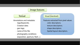
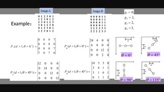
16. • The GLCM is defined by:
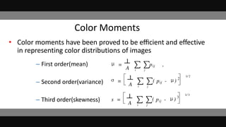
– wherenij is the number of occurrences of the pixel
values lying at distance d with angle  in the image.
– The co-occurrence matrix P has dimension n x n,
where n is the number of gray levels in the image.
P(p,q,d,)  nij
#{[(x , y ),(x , y )]S | f (x , y )  p & f (x , y )  q}
p(p,q,d,)  1 1 2 2 1 1 2 2
#S
GLCM
(p,q)
nij

17. Example：
0 1 2 3 0 1
1 2 3 0 1 2
2 3 0 1 2 3
3 0 1 2 3 0
0 1 2 3 0 1
1 2 3 0 1 2
0 0 0 0 1 1
0 0 0 0 1 1
0 0 0 0 1 1
0 0 0 0 1 1
2 2 2 2 3 3
2 2 2 2 3 3
ImageA Image B
0 8 0 7
8 0 8 0
0 8 0 7
7 0 7 0
P (d  1,  0 )
o
A 
g1  0,
g2  1,
g3  2,
g4  3,
  0o   45o
  90o
  135o
P (d  1,  45o
) 
B
18 3 3 0
3
3
6
1
1
6
1
1
0 1 1 2
P (d  1,  45o
) 
A
12 0 0 0
0
0
14
0
0
12
0
0
0 0 0 12
P (d  1,  0o
) 
B
24 4 0 0
4
0
8
0
0
12
0
2
0 0 2 4

18.  Gray Level Co-occurrence Matrix
 Contains information about the positions of
pixels having similar gray level values.
 Robust to translation and rotation about the
view axis and changes only slowly with the
scale, occlusion and viewing angle.
GLCM

19. Popular Visual Features
 Global Feature
– Color
Color space
Color histogram
Color moment
– Texture
GLCM
– Shape Context
– GIST
– Color Name
 Local Feature
– Detector
Harris, LOG, DOG, MSER, Hessian Affine
KAZE, FAST
– Descriptor
SIFT, SURF, LIOP, BRIEF
ORB, FREAK, BRISK, CARD, Edge-SIFT

20. • What points on these two sampled contours are
most similar? How do you know?

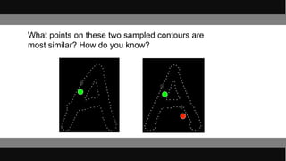
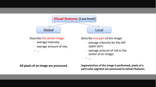
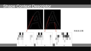
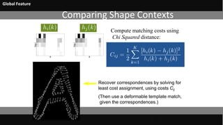
21. Shape Context Descriptor [Belongie et al ’02]
20
Shape context slides from Belongie et al.
Count the number of points
inside each bin, e.g.:
Count = 4
Count = 10
Compact representation of
distribution of points relative
to each point
...
NIPS’00, PAMI’02

22. Shape Context Descriptor
形状直方图

23. Global Feature
Comparing Shape Contexts
22
Compute matching costs using
Chi Squared distance:
Recover correspondences by solving for
least cost assignment, using costs Cij
(Then use a deformable template match,
given the correspondences.)

24. Popular Visual Features
 Global Feature
– Color
Color space
Color histogram
Color moment
– Texture
GLCM
– Shape Context
– GIST
– Color Name
 Local Feature
– Detector
Harris, LOG, DOG, MSER, Hessian Affine
KAZE, FAST
– Descriptor
SIFT, SURF, LIOP, BRIEF
ORB, FREAK, BRISK, CARD, Edge-SIFT

25. GIST Feature
• Definition and Background
• Essence, holistic characteristics of an image
• Context information obtained within an eye saccade (app.
150 ms.)
• Evidence of place recognizing cells at Parahippocampal
Place Area (PPA)
• Biologically plausible models of Gist are yet to be
proposed
• Nature of tasks done with gist
• Scene categorization/context recognition
• Region priming/layout recognition
• Resolution/scale selection
C. Siagian and L. I t , Rapid Biologically-‐Inspired Scene ClassificaOon Using Features Shared with
Visual AuenOon, IEEE Transac=ons PAMI, Vol. 29, No. 2, pp. 300-‐312, Feb 2007.
C. Siagian and L. Itti, Rapid Biologically‐Inspired Scene Classification Using Features Shared with Visual Attention,
IEEE Transactions on PAMI, Vol.29,No.2,pp.300-312,Feb 2007.

26. Human Vision Architecture
• Visual Cortex:
– Low level filters, center-surround,
and normalization
• Saliency Model:
– Attend to pertinent regions
• Gist Model:
– Compute image general
characteristic
• High Level Vision:
– Object recognition
– Layout recognition
– Scene understanding

27. Gist Model Implementation
 Raw image feature-maps
• Gabor filters at 4 angles (0,
45, 90, 135) on 4 scales
= 16 sub-‐channels
• red-‐green and blue-‐yellow center
surround each with 6 scale
combinations
= 12 sub-‐channels
• Dark-bright center-surround with 6
scale combinations
= 6 sub-‐channels
= Total of 34 sub-‐channels
 Orientation Channel
 color
 Intensity

28. Gist Model Implementation
• Gist Feature Extraction
– Average values of predetermined grid （4×4）
Global Feature

29. • Dimension Reduction
– Original:
34 sub-‐channels x 16
features
= 544 features
– PCA/ICA reduction: 80
features
• Kept >95% of variance
Gist Model Implementation
Global Feature

30. System Example
Run

31. Global Features
• Advantages:
– Simple.
– Low computatinal complexity.
• Disadvantages:
– Low accuracy

32. • Why Local Feature?
– Locality: features are local, so robust to occlusion
and clutter (no prior segmentation)
– Distinctiveness: individual features can be matched
to a large database of objects
– Quantity: many features can be generated for even
small objects
– Efficiency: close to real-time performance
– Extensibility: can easily be extended to wide range of
differing feature types, with each adding robustness
Local Features

33. • Main Components:
– Detection of interest points
– Local Feature Descriptor
Local Features
Image Interest Points Local Feature

34. Popular Visual Features
 Global Feature
– Color
Color space
Color histogram
Color moment
– Texture
GLCM
– Shape Context
– GIST
– Color Name
 Local Feature
– Detector
Harris, LOG, DOG, MSER, Hessian Affine
KAZE, FAST
– Descriptor
SIFT, SURF, LIOP, BRIEF
ORB, FREAK, BRISK, CARD, Edge-SIFT

35. Local Feature
• Corners as distinctive interest points
− We should easily recognize the point by looking through a
small window
− shift a window in any direction should give a large change in
intensity
“Flat” Region:
No change in all
direction
“Edge”:
No change along the
edge direction
“Corner”: Significant
Change in all directions
Harris Corner Detector

36. Consider shifting the window W by (u,v)
• how do the pixels in W change?
• compare each pixel before and after by
summing up the squared differences W
Taylor Series expansion of I:
If the motion (u,v) is small, then first order approx is good
Local Feature
Harris Corner Detector

37. W
Local Feature
Harris Corner Detector

38. M
This can be rewritten as
For the example above
• You can move the center of the blue window to anywhere on the
yellow unit circle
• Which directions will result in the largest and smallest E values?
• We can find these directions by looking at the eigenvectors of M
Local Feature
Harris Corner Detector

39. Eigenvalues and eigenvectors of M
• Define shifts with the smallest and largest change (E value)
•
•
•
•
x+ = direction of largest increase in E.
+ = amount of increase in direction x+
x- = direction of smallest increase in E.
-‐= amount of increase in direction x-
x-
x+
M
Mx   x
Mx   x  
Local Feature
Harris Corner Detector

40. “Flat” Region:
λ1 and λ2 are small;
“Edge”:
λ1 >> λ2
λ2 >> λ1
“Corner”:
λ1 and λ2 are large;
λ1 ~ λ2
Local Feature
Harris Corner Detector

41. Feature Detection: Mathematics
1
2
“Corner”
1 and 2 are large,
1 ~ 2;
E increases in all
directions
1 and 2 are small; E
is almost constant in
all directions
“Edge”
1 >> 2
“Edge”
2 >> 1
“Flat”
region
Classification of image
points using eigenvalues
of M:
12
1  2
f  2
f  12 (1  2 )Corner Response Function: or

42. Harris Corner Detector
• Procedure:
− Compute M matrix for each image window to get their
cornerness scores
− Find points whose surrounding window gave large corner
response
− Take the points of local maxima, i.e., perform non
-‐maximum suppression
优点：A 、旋转不变性；B、图像灰度的仿射变化具有部分的不变性。
缺点：A 、它对尺度很敏感，不具备几何尺度不变性；B、提取的角点是像素级的。

43. Harris Detector Example

44. The tops of the horns are detected in both images
Harris Corner (in red)

45. Popular Visual Features
 Global Feature
– Color
Color space
Color histogram
Color moment
– Texture
GLCM
– Shape Context
– GIST
– Color Name
 Local Feature
– Detector
Harris, LOG, DOG, MSER, Hessian Affine
KAZE, FAST
– Descriptor
SIFT, SURF, LIOP, BRIEF
ORB, FREAK, BRISK, CARD, Edge-SIFT

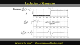
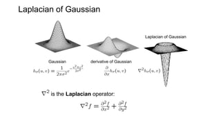
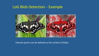
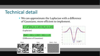
46. Laplacian of Gaussian
 LoG边缘检测算子是David Courtnay Marr和Ellen Hildreth（1980）共
同提出的[1] 。因此，也称为边缘检测算法或Marr & Hildreth算子。
 该算法首先对图像做高斯滤波，然后再求其拉普拉斯（Laplacian）二阶导
数。即图像与 Laplacian of the Gaussian function 进行滤波运算。最后，
通过检测滤波结果的零交叉（Zero crossings）可以获得图像或物体的边
缘。因而，也被业界简称为Laplacian-of-Gaussian (LoG)算子。

47. Laplacian of Gaussian
Consider
Laplacian of Gaussian
operator
Where is the edge? Zero-crossings of bottom graph

48. is the Laplacian operator:
Laplacian of Gaussian
Gaussian derivative of Gaussian
Laplacian of Gaussian

49. Laplacian-‐of-‐Gaussian (LoG)
We define the characteristic scale as the scale
that produces peak of Laplacian response.

50. Laplacian of Gaussian

51. LoG Blob Detection -‐ Example
Interest points can be defined as the centers of blobs.

52. Popular Visual Features
 Global Feature
– Color
Color space
Color histogram
Color moment
– Texture
GLCM
– Shape Context
– GIST
– Color Name
 Local Feature
– Detector
Harris, LOG, DOG, MSER, Hessian Affine
KAZE, FAST
– Descriptor
SIFT, SURF, LIOP, BRIEF
ORB, FREAK, BRISK, CARD, Edge-SIFT

53. Technical detail
 We can approximate the Laplacian with a difference
of Gaussians; more efficient to implement.
(Laplacian)
(Difference of Gaussians)

54. DoG Image Pyramid
0 02 

55. , 0 2o ks
o s  

, 0 2ks
o s 

56. Local Extrema Detection
 Maxima and minima
 Compare x with its 26
neighbors at 3 scales

57. D(x, y, σ) = (G(x,y, kσ) − G(x,y, σ)) ∗ I(x, y) = L(x,y, kσ) − L(x,y, σ).

58. Popular Visual Features
 Global Feature
– Color
Color space
Color histogram
Color moment
– Texture
GLCM
– Shape Context
– GIST
– Color Name
 Local Feature
– Detector
Harris, LOG, DOG, MSER, Hessian Affine
KAZE, FAST
– Descriptor
SIFT, SURF, GLOH, LIOP, BRIEF
ORB, FREAK, BRISK, CARD, Edge-SIFT

59. SIFT Descriptor
• Making descriptor rotation invariant
• Rotate patch according to its dominant gradient orientation
• This puts patches into a canonical orientation.
Local Feature

60. Scale Invariant Feature Transform
(SIFT) descriptor
• Basic idea:
− Take 16x16 square window around detected feature
− Compute edge orientation (angle of the gradient -‐90) for
each pixel
− Throw out weak edges (threshold gradient magnitude)
− Create histogram of surviving edge orientations
0 2
angle histogram

61. Orientation
Gradient and angle:
2 2
m(x, y)  L(x 1, y)  L(x 1, y) L(x, y 1)  L(x, y 1)
(x, y)  tan1
L(x, y 1) L(x, y 1)/ L(x 1, y)  L(x 1, y)
Orientation selection

62. • Full version:
− Divide the 16x16 window into a 4x4 grid of cells (2x2 case
shown below)
− Compute an orientation histogram for each cell
− 16 cells X 8 orientations = 128 dimensional descriptor
Scale Invariant Feature Transform
(SIFT) descriptor

63. • Invariant to
– Scale
– Rotation
• Partially invariant to
– Illumination changes
– Camera viewpoint
– Occlusion, clutter
Scale Invariant Feature Transform
(SIFT) descriptor

64. Popular Visual Features
 Global Feature
– Color
Color space
Color histogram
Color moment
– Texture
GLCM
– Shape Context
– GIST
– Color Name
 Local Feature
– Detector
Harris, LOG, DOG, MSER, Hessian Affine
KAZE, FAST
– Descriptor
SIFT, SURF, GLOH, LIOP, BRIEF
ORB, FREAK, BRISK, CARD, Edge-SIFT

65. SURF: Speeded Up Robust Features
• Using integral images for major speed up
– Integral Image (summed area tables) is an intermediate represention for the
image and contains the sum of gray scale pixel values of image
– They allow for fast computation of box type convolution filters.
ECCV 2006, CVIU 2008
• SURF角点检测算法是对SIFT的一种改进，主要体现在速度上，效率更高。
它和SIFT的主要区别是图像多尺度空间的构建方法不同。

66. SURF
A comparison of SIFT, PCA-SIFT and SURF
method Time Scale Rotation Blur Illumination Affine
Sift common best best common common good
PCA-sift good good good best good best
Surf best common common good best good

67. 108
• Hessian-‐based interest point localization
• Lxx(x,y,σ) is the Laplacian of Gaussian of the image
• It is the convolution of the Gaussian second order
derivative with the image
构造高斯金字塔尺度空间
SURF

68. 110
• Approximated second order derivative with box
filters (mean/average filter)
Local Feature
SURF
利用模板求偏导和卷积，得到hessian行列式图，类比于sift中的DOG图

69. 111
Detection
• Scale analysis with constant image size
9 x 9, 15 x 15, 21 x 21, 27 x 27  39 x 39, 51 x 51 …
1st octave 2nd octave
Local Feature

70. 113
Description
• Orientation Assignment
Circular neighborhood of
radius 6s around the interest point
(s = the scale at which the point was detected)
Side length = 4s Cost 6
operation to compute
the response
x response y response
Local Feature
与sift不同，surf是统计60度扇形内所
有点的水平haar小波特征和垂直haar小
波特征总和

71. Popular Visual Features
 Global Feature
– Color
Color space
Color histogram
Color moment
– Texture
GLCM
– Shape Context
– GIST
– Color Name
 Local Feature
– Detector
Harris, LOG, DOG, MSER, Hessian Affine
KAZE, FAST
– Descriptor
SIFT, SURF, GLOH, LIOP, BRIEF
ORB, FREAK, BRISK, CARD, Edge-SIFT

72. GLOH : Gradient location-orientation histogram
(Mikolajczyk and Schmid 2005)
16-bin location-orientation bin histogram -> 272D -> 128D by PCA
SIFT GLOH
Local Feature
使用对数极坐标分级结构替代 SIFT 使用的4象限。
空间上取半径6，11，15，角度上分八个区间（除中间
区域）,然后将272（17*16）维的histogram在一个大数
据库上训练，用PCA投影到一个128维向量

73. Popular Visual Features
 Global Feature
– Color
Color space
Color histogram
Color moment
– Texture
GLCM
– Shape Context
– GIST
– Color Name
 Local Feature
– Detector
Harris, LOG, DOG, MSER, Hessian Affine
KAZE, FAST
– Descriptor
SIFT, SURF, GLOH, LIOP, BRIEF
ORB, FREAK, BRISK, CARD, Edge-SIFT

74.  Zhenhua Wang, Bin Fan, and Fuchao Wu,
"Local intensity order pattern for feature
description." ICCV, 2011
 Motivation: Orientation estimation error in SIFT
LIOP

75. LIOP: Local intensity order pattern for
feature description

76. Popular Visual Features
 Global Feature
– Color
Color space
Color histogram
Color moment
– Texture
GLCM
– Shape Context
– GIST
– Color Name
 Local Feature
– Detector
Harris, LOG, DOG, MSER, Hessian Affine
KAZE, FAST
– Descriptor
SIFT, SURF, GLOH, LIOP, BRIEF
ORB, FREAK, BRISK, CARD, Edge-SIFT

77. Edge-SIFT

IEEE TIP-‐2014
: discriminative binary descriptor for scalable
partial-duplicate mobile search.
Histogram based descriptor:
• Good for classification tasks,
• Expensive, not optimal for partial-duplicate search
Motivation—the edge map:
• preserves structural clue and spatial clue
• sparse, fast to compute
• Is potential for local descriptor extraction


78. Extraction of Edge-SIFT
0-degree 45-degree 90-degree 135-degree
884  256bit descriptor
da
S
Orientation
S
S
Edge Extraction&EdgeDescriptor Computation
S
scale
db
Orientation
scale
Keypoint Detection Image Patch Extraction&Normalization

79. The Matching Performance
The matching result of SIFT
The matching result of Edge-SIFT

80. Thank you !