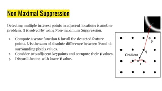
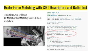
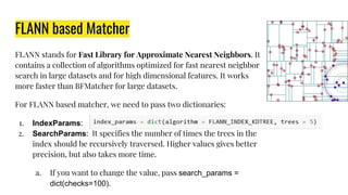
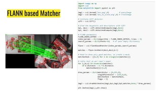
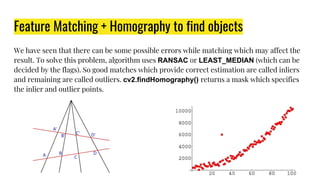
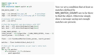
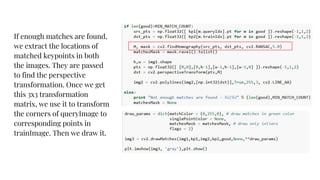
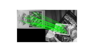
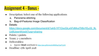
Practical 4 - Digital Image
Processing
Aly Osama
‫درﯾد‬ ‫اﺑن‬
‫ﯾـرى‬ ‫ِﻣـﺎ‬‫ﺑ‬ ُ‫ه‬َ‫َـر‬‫ﯾ‬ ‫َم‬‫ﻟ‬ ‫ﻣﺎ‬ َ‫ﻗﺎس‬ ‫َن‬‫ﻣ‬
‫َـﺄى‬‫ﻧ‬ ‫ﻣـﺎ‬ ِ‫ﮫ‬‫َﯾـ‬‫ﻟ‬ِ‫إ‬ ‫َدﻧـو‬‫ﯾ‬ ‫ﻣـﺎ‬ ُ‫ه‬‫َرا‬‫أ‬
Stages of Computer Vision
Agenda
1. Intro to feature descriptors
2. Harris Corner Detection
3. Introduction to SIFT
4. Introduction to SURF
5. FAST
6. BRIEF
7. ORB (Oriented FAST and Rotated BRIEF)
8. Feature Matching
9. Feature Matching + Homography to find Objects
10. Assignment
11. Project
Intro to Feature Detection
Understanding Features
We are looking for specific patterns or specific
features which are unique, which can be easily
tracked, which can be easily compared.
A and B are flat surfaces, and they are spread in a lot
of area. It is difficult to find the exact location of
these patches.
C and D are much more simpler. They are edges of
the building. You can find an approximate location,
but exact location is still difficult. It is because,
along the edge, it is same everywhere. Normal to the
edge, it is different. So edge is a much better feature
compared to flat area, but not good enough.
Understanding Features
Finally, E and F are some corners of the building.
And they can be easily found out. Because at
corners, wherever you move this patch, it will look
different. So they can be considered as a good
feature.
Harris Corner Detection
Harris Corner Detector
Theory
It basically finds the difference in intensity for a displacement of (u,v) in all directions.
We have to maximize this function E(u,v) for corner detection. That means, we have to maximize the
second term. So, applying Taylor Expansion to above equation and using some mathematical steps
where
Ix and Iy are image derivatives in
x and y directions respectively. (Can
be easily found out using
cv2.Sobel()).
Harris Corner Detector
This equation will determine if a window can contain a corner or not.
Harris Corner Detector in OpenCV
OpenCV has the function cv2.cornerHarris() for this purpose. Its arguments are :
● img - Input image, it should be grayscale and float32 type.
● blockSize - It is the size of neighbourhood considered for corner detection
● ksize - Aperture parameter of Sobel derivative used.
● k - Harris detector free parameter in the equation.
dst = cv2.cornerHarris(gray,2,3,0.04)
SIFT (Scale-Invariant
Feature Transform)
SIFT
Theory
We saw some corner detectors like Harris etc. They are rotation-invariant, which means,
even if the image is rotated, we can find the same corners. But what about scaling? A
corner may not be a corner if the image is scaled.
Scale Invariant Feature Transform (SIFT) extracts keypoints and compute its descriptors
SIFT
SIFT Algorithm
SIFT is quite an involved algorithm. It has a lot going on and can become confusing, So I've split up the entire algorithm into
multiple parts. Here's an outline of what happens in SIFT.
1. Constructing a scale space
2. LoG Approximation
3. Finding keypoints
4. Get rid of bad key points
5. Assigning an orientation to the keypoints
6. Generate SIFT features
More details: http://aishack.in/tutorials/sift-scale-invariant-feature-transform-introduction/
SIFT - 1)Constructing a scale space
This is the initial preparation. You create
internal representations of the original image
to ensure scale invariance. This is done by
generating a "scale space".
SIFT - 2) LoG approximation
The Laplacian of Gaussian is great for finding
interesting points (or key points) in an image. But
it's computationally expensive. So we cheat and
approximate it using the representation created
earlier
SIFT 3) Finding Keypoints
With the super fast approximation, we now try to
find key points. These are maxima and minima in
the Difference of Gaussian image we calculate in
step 2
SIFT 4) Get rid of bad key points
Edges and low contrast
regions are bad keypoints.
Eliminating these makes the
algorithm efficient and robust.
A technique similar to the
Harris Corner Detector is used
here
SIFT 5) Assigning an orientation to key points
an orientation is calculated for each
key point. Any further calculations
are done relative to this orientation.
This effectively cancels out the effect
of orientation, making it rotation
invariant.
SIFT 6) Generate features
Finally, with scale and rotation invariance in
place, one more representation is generated.
This helps uniquely identify features. Lets say
you have 50,000 features. With this
representation, you can easily identify the feature
you're looking for (say, a particular eye, or a sign
board). That was an overview of the entire
algorithm.
SIFT in OpenCV
OpenCV also provides cv2.drawKeyPoints()
function which draws the small circles on the
locations of keypoints.
SIFT in OpenCV
Now to calculate the descriptor, OpenCV provides two methods.
1. Since you already found key points, you can call sift.compute() which computes the
descriptors from the keypoints we have found.
2. If you didn’t find keypoints, directly find keypoints and descriptors in a single step
with the function, sift.detectAndCompute().
SURF (Speeded-Up Robust
Features)
SURF
Theory
SIFT was comparatively slow and people needed more speeded-up
version. a new algorithm called SURF introduced, it is a
speeded-up version of SIFT.
In short, SURF adds a lot of
features to improve the speed in
every step. Analysis shows it is 3
times faster than SIFT while
performance is comparable to
SIFT. SURF is good at handling
images with blurring and rotation,
but not good at handling viewpoint
change and illumination change.
SURF in OpenCV
You initiate a SURF object with some optional conditions like 400-dim
descriptors, Upright/Normal SURF etc.
699 keypoints is too much to show in a picture. We reduce it to some 50 to draw
it on an image. While matching, we may need all those features, but not now. So
we increase the Hessian Threshold.
It is less than 50. Let’s draw it on the image.
FAST Algorithm for Corner
Detection
FAST - Theory
We saw several feature detectors and many of
them are really good. But when looking from a
real-time application point of view, they are not
fast enough. One best example would be SLAM
(Simultaneous Localization and Mapping) mobile
robot which have limited computational
resources.
As a solution to this, FAST (Features from
Accelerated Segment Test) algorithm was
proposed by Edward Rosten and Tom Drummond
in their paper “Machine learning for high-speed
corner detection” .
Feature Detection using FAST
1. Select a pixel Ƥ in the image which is to be
identified as an interest point or not. Let its
intensity be
2. Select appropriate threshold value ʈ
3. Consider a circle of 16 pixels around the pixel
under test.
4. Now the pixel Ƥ is a corner if there exists a
set of ɳ (chosen to be 12) contiguous pixels in
the circle (of 16 pixels) which are all brighter
than
5. A high-speed test was proposed to exclude a
large number of non-corners.
Machine Learning a Corner Detector
1. Select a set of images for training
2. For every feature point, store the 16 pixels around it as a vector. Do it for all the images to
get feature vector P.
3. Each pixel (say ) in these 16 pixels can have one of the following three states:
5. Depending on these states, the feature vector P is subdivided into 3 subsets,
6. Define a new boolean variable, which is true if Ƥ is a corner and false otherwise.
7. Use the ID3 algorithm (decision tree classifier) to query each subset using the variable
for the knowledge about the true class. It selects the which yields the most information
about whether the candidate pixel is a corner, measured by the entropy of
8. This is recursively applied to all the subsets until its entropy is zero.
9. The decision tree so created is used for fast detection in other images
Non Maximal Suppression
Detecting multiple interest points in adjacent locations is another
problem. It is solved by using Non-maximum Suppression.
1. Compute a score function for all the detected feature
points. is the sum of absolute difference between Ƥ and 16
surrounding pixels values.
2. Consider two adjacent keypoints and compute their values.
3. Discard the one with lower value.
It is several times faster than other
existing corner detectors.
But it is not robust to high levels of
noise. It is dependant on a
threshold.
FAST with OpenCV
BRIEF (Binary Robust
Independent Elementary
Features)
BRIEF
Theory
We know SIFT uses 128-dim vector for descriptors. Since it is using floating point numbers, it
takes basically 512 bytes. Similarly SURF also takes minimum of 256 bytes (for 64-dim). Creating
such a vector for thousands of features takes a lot of memory which are not feasible for
resource-constraint applications especially for embedded systems. Larger the memory, longer
the time it takes for matching. But all these dimensions may not be needed for actual matching.
BRIEF
We can compress it using several methods like PCA, LDA etc. Even other methods like hashing
using LSH (Locality Sensitive Hashing) is used to convert these SIFT descriptors in floating point
numbers to binary strings.
These binary strings are used to match features using Hamming distance. This provides better
speed-up because finding hamming distance is just applying XOR and bit count, which are very
fast in modern CPUs with SSE instructions. But here, we need to find the descriptors first, then
only we can apply hashing, which doesn’t solve our initial problem on memory.
In short, BRIEF is a faster method feature descriptor calculation and matching. It also provides
high recognition rate unless there is large in-plane rotation.
BRIEF in OpenCV
ORB (Oriented FAST and
Rotated BRIEF)
ORB
It is a good alternative to SIFT and SURF in computation
cost, matching performance and mainly the patents.
ORB is basically a fusion of FAST keypoint detector and
BRIEF descriptor with many modifications to enhance the
performance.
● First it use FAST to find keypoints,
● then apply Harris corner measure to find top N
points among them.
● It also use pyramid to produce multiscale-features.
ORB in OpenCV
Feature Matching
Basics of Brute-Force matcher
Brute-Force matcher is simple. It takes the descriptor of one feature in first set
and is matched with all other features in second set using some distance
calculation. And the closest one is returned.
Brute-Force matcher with ORB descriptors
Here, we will see a simple example on how to match features between two
images
Brute-Force matcher with ORB descriptors
What is Matcher object?
The result of matches = bf.match(des1,des2) line is a list of DMatch objects. This
DMatch object has following attributes:
● DMatch.distance - Distance between descriptors. The lower, the better it is.
● DMatch.trainIdx - Index of the descriptor in train descriptors
● DMatch.queryIdx - Index of the descriptor in query descriptors
● DMatch.imgIdx - Index of the train image.
Brute-Force Matching with SIFT Descriptors and Ratio Test
This time, we will use
BFMatcher.knnMatch() to get k best
matches.
FLANN based Matcher
FLANN stands for Fast Library for Approximate Nearest Neighbors. It
contains a collection of algorithms optimized for fast nearest neighbor
search in large datasets and for high dimensional features. It works
more faster than BFMatcher for large datasets.
For FLANN based matcher, we need to pass two dictionaries:
1. IndexParams:
2. SearchParams: It specifies the number of times the trees in the
index should be recursively traversed. Higher values gives better
precision, but also takes more time.
a. If you want to change the value, pass search_params =
dict(checks=100).
FLANN based Matcher
Feature Matching +
Homography to find Objects
Feature Matching + Homography to find objects
We have seen that there can be some possible errors while matching which may affect the
result. To solve this problem, algorithm uses RANSAC or LEAST_MEDIAN (which can be
decided by the flags). So good matches which provide correct estimation are called inliers
and remaining are called outliers. cv2.findHomography() returns a mask which specifies
the inlier and outlier points.
Now we set a condition that at least 10
matches (defined by
MIN_MATCH_COUNT) are to be there
to find the object. Otherwise simply
show a message saying not enough
matches are present.
If enough matches are found,
we extract the locations of
matched keypoints in both
the images. They are passed
to find the perspective
transformation. Once we get
this 3x3 transformation
matrix, we use it to transform
the corners of queryImage to
corresponding points in
trainImage. Then we draw it.
Assignment
Assignment 4 - Bonus -
● Description: Select one of the following applications
a. Panorama stitching
b. Bag-of-Features Image Classification
● Details:
https://docs.google.com/document/d/1ahS-YFY2ocGiLxhFdMrutTlI8vYEu33_9L
Ud8Uewr4A/edit?usp=sharing
● Points: 5 points
● Team: 2-3 members
● Deliverables:
a. Jupyter (html) notebook to https://goo.gl/forms/yhnMiSKaz7goFVyA3
● Deadline: 17th April 2018
Project
Project
● Our competition has 65 teams
● Deadline: 30th April.
Have a question?!
If you have any question
● Facebook
○ You can ask me through Facebook but don’t wait for any response before 1 month.
“Simply don’t use facebook”
● Office Hours
○ Monday 3:30 to 5:00
○ Wednesday 11:30 to 12:30
● Email (Prefered)
○ aly.osama@eng.asu.edu.eg
Thank you

Practical Digital Image Processing 4

  • 1.
    Practical 4 -Digital Image Processing Aly Osama
  • 2.
    ‫درﯾد‬ ‫اﺑن‬ ‫ﯾـرى‬ ‫ِﻣـﺎ‬‫ﺑ‬ُ‫ه‬َ‫َـر‬‫ﯾ‬ ‫َم‬‫ﻟ‬ ‫ﻣﺎ‬ َ‫ﻗﺎس‬ ‫َن‬‫ﻣ‬ ‫َـﺄى‬‫ﻧ‬ ‫ﻣـﺎ‬ ِ‫ﮫ‬‫َﯾـ‬‫ﻟ‬ِ‫إ‬ ‫َدﻧـو‬‫ﯾ‬ ‫ﻣـﺎ‬ ُ‫ه‬‫َرا‬‫أ‬
  • 3.
  • 4.
    Agenda 1. Intro tofeature descriptors 2. Harris Corner Detection 3. Introduction to SIFT 4. Introduction to SURF 5. FAST 6. BRIEF 7. ORB (Oriented FAST and Rotated BRIEF) 8. Feature Matching 9. Feature Matching + Homography to find Objects 10. Assignment 11. Project
  • 5.
  • 7.
    Understanding Features We arelooking for specific patterns or specific features which are unique, which can be easily tracked, which can be easily compared. A and B are flat surfaces, and they are spread in a lot of area. It is difficult to find the exact location of these patches. C and D are much more simpler. They are edges of the building. You can find an approximate location, but exact location is still difficult. It is because, along the edge, it is same everywhere. Normal to the edge, it is different. So edge is a much better feature compared to flat area, but not good enough.
  • 8.
    Understanding Features Finally, Eand F are some corners of the building. And they can be easily found out. Because at corners, wherever you move this patch, it will look different. So they can be considered as a good feature.
  • 9.
  • 10.
    Harris Corner Detector Theory Itbasically finds the difference in intensity for a displacement of (u,v) in all directions. We have to maximize this function E(u,v) for corner detection. That means, we have to maximize the second term. So, applying Taylor Expansion to above equation and using some mathematical steps where Ix and Iy are image derivatives in x and y directions respectively. (Can be easily found out using cv2.Sobel()).
  • 11.
    Harris Corner Detector Thisequation will determine if a window can contain a corner or not.
  • 12.
    Harris Corner Detectorin OpenCV OpenCV has the function cv2.cornerHarris() for this purpose. Its arguments are : ● img - Input image, it should be grayscale and float32 type. ● blockSize - It is the size of neighbourhood considered for corner detection ● ksize - Aperture parameter of Sobel derivative used. ● k - Harris detector free parameter in the equation. dst = cv2.cornerHarris(gray,2,3,0.04)
  • 14.
  • 15.
    SIFT Theory We saw somecorner detectors like Harris etc. They are rotation-invariant, which means, even if the image is rotated, we can find the same corners. But what about scaling? A corner may not be a corner if the image is scaled. Scale Invariant Feature Transform (SIFT) extracts keypoints and compute its descriptors
  • 16.
  • 18.
    SIFT Algorithm SIFT isquite an involved algorithm. It has a lot going on and can become confusing, So I've split up the entire algorithm into multiple parts. Here's an outline of what happens in SIFT. 1. Constructing a scale space 2. LoG Approximation 3. Finding keypoints 4. Get rid of bad key points 5. Assigning an orientation to the keypoints 6. Generate SIFT features More details: http://aishack.in/tutorials/sift-scale-invariant-feature-transform-introduction/
  • 19.
    SIFT - 1)Constructinga scale space This is the initial preparation. You create internal representations of the original image to ensure scale invariance. This is done by generating a "scale space".
  • 20.
    SIFT - 2)LoG approximation The Laplacian of Gaussian is great for finding interesting points (or key points) in an image. But it's computationally expensive. So we cheat and approximate it using the representation created earlier
  • 21.
    SIFT 3) FindingKeypoints With the super fast approximation, we now try to find key points. These are maxima and minima in the Difference of Gaussian image we calculate in step 2
  • 22.
    SIFT 4) Getrid of bad key points Edges and low contrast regions are bad keypoints. Eliminating these makes the algorithm efficient and robust. A technique similar to the Harris Corner Detector is used here
  • 23.
    SIFT 5) Assigningan orientation to key points an orientation is calculated for each key point. Any further calculations are done relative to this orientation. This effectively cancels out the effect of orientation, making it rotation invariant.
  • 24.
    SIFT 6) Generatefeatures Finally, with scale and rotation invariance in place, one more representation is generated. This helps uniquely identify features. Lets say you have 50,000 features. With this representation, you can easily identify the feature you're looking for (say, a particular eye, or a sign board). That was an overview of the entire algorithm.
  • 25.
    SIFT in OpenCV OpenCValso provides cv2.drawKeyPoints() function which draws the small circles on the locations of keypoints.
  • 26.
    SIFT in OpenCV Nowto calculate the descriptor, OpenCV provides two methods. 1. Since you already found key points, you can call sift.compute() which computes the descriptors from the keypoints we have found. 2. If you didn’t find keypoints, directly find keypoints and descriptors in a single step with the function, sift.detectAndCompute().
  • 27.
  • 28.
    SURF Theory SIFT was comparativelyslow and people needed more speeded-up version. a new algorithm called SURF introduced, it is a speeded-up version of SIFT.
  • 29.
    In short, SURFadds a lot of features to improve the speed in every step. Analysis shows it is 3 times faster than SIFT while performance is comparable to SIFT. SURF is good at handling images with blurring and rotation, but not good at handling viewpoint change and illumination change.
  • 30.
    SURF in OpenCV Youinitiate a SURF object with some optional conditions like 400-dim descriptors, Upright/Normal SURF etc. 699 keypoints is too much to show in a picture. We reduce it to some 50 to draw it on an image. While matching, we may need all those features, but not now. So we increase the Hessian Threshold.
  • 31.
    It is lessthan 50. Let’s draw it on the image.
  • 32.
    FAST Algorithm forCorner Detection
  • 33.
    FAST - Theory Wesaw several feature detectors and many of them are really good. But when looking from a real-time application point of view, they are not fast enough. One best example would be SLAM (Simultaneous Localization and Mapping) mobile robot which have limited computational resources. As a solution to this, FAST (Features from Accelerated Segment Test) algorithm was proposed by Edward Rosten and Tom Drummond in their paper “Machine learning for high-speed corner detection” .
  • 34.
    Feature Detection usingFAST 1. Select a pixel Ƥ in the image which is to be identified as an interest point or not. Let its intensity be 2. Select appropriate threshold value ʈ 3. Consider a circle of 16 pixels around the pixel under test. 4. Now the pixel Ƥ is a corner if there exists a set of ɳ (chosen to be 12) contiguous pixels in the circle (of 16 pixels) which are all brighter than 5. A high-speed test was proposed to exclude a large number of non-corners.
  • 35.
    Machine Learning aCorner Detector 1. Select a set of images for training 2. For every feature point, store the 16 pixels around it as a vector. Do it for all the images to get feature vector P. 3. Each pixel (say ) in these 16 pixels can have one of the following three states: 5. Depending on these states, the feature vector P is subdivided into 3 subsets, 6. Define a new boolean variable, which is true if Ƥ is a corner and false otherwise. 7. Use the ID3 algorithm (decision tree classifier) to query each subset using the variable for the knowledge about the true class. It selects the which yields the most information about whether the candidate pixel is a corner, measured by the entropy of 8. This is recursively applied to all the subsets until its entropy is zero. 9. The decision tree so created is used for fast detection in other images
  • 36.
    Non Maximal Suppression Detectingmultiple interest points in adjacent locations is another problem. It is solved by using Non-maximum Suppression. 1. Compute a score function for all the detected feature points. is the sum of absolute difference between Ƥ and 16 surrounding pixels values. 2. Consider two adjacent keypoints and compute their values. 3. Discard the one with lower value.
  • 37.
    It is severaltimes faster than other existing corner detectors. But it is not robust to high levels of noise. It is dependant on a threshold.
  • 38.
  • 39.
  • 40.
    BRIEF Theory We know SIFTuses 128-dim vector for descriptors. Since it is using floating point numbers, it takes basically 512 bytes. Similarly SURF also takes minimum of 256 bytes (for 64-dim). Creating such a vector for thousands of features takes a lot of memory which are not feasible for resource-constraint applications especially for embedded systems. Larger the memory, longer the time it takes for matching. But all these dimensions may not be needed for actual matching.
  • 41.
    BRIEF We can compressit using several methods like PCA, LDA etc. Even other methods like hashing using LSH (Locality Sensitive Hashing) is used to convert these SIFT descriptors in floating point numbers to binary strings. These binary strings are used to match features using Hamming distance. This provides better speed-up because finding hamming distance is just applying XOR and bit count, which are very fast in modern CPUs with SSE instructions. But here, we need to find the descriptors first, then only we can apply hashing, which doesn’t solve our initial problem on memory. In short, BRIEF is a faster method feature descriptor calculation and matching. It also provides high recognition rate unless there is large in-plane rotation.
  • 42.
  • 43.
    ORB (Oriented FASTand Rotated BRIEF)
  • 44.
    ORB It is agood alternative to SIFT and SURF in computation cost, matching performance and mainly the patents. ORB is basically a fusion of FAST keypoint detector and BRIEF descriptor with many modifications to enhance the performance. ● First it use FAST to find keypoints, ● then apply Harris corner measure to find top N points among them. ● It also use pyramid to produce multiscale-features.
  • 45.
  • 46.
  • 48.
    Basics of Brute-Forcematcher Brute-Force matcher is simple. It takes the descriptor of one feature in first set and is matched with all other features in second set using some distance calculation. And the closest one is returned.
  • 49.
    Brute-Force matcher withORB descriptors Here, we will see a simple example on how to match features between two images
  • 50.
    Brute-Force matcher withORB descriptors
  • 51.
    What is Matcherobject? The result of matches = bf.match(des1,des2) line is a list of DMatch objects. This DMatch object has following attributes: ● DMatch.distance - Distance between descriptors. The lower, the better it is. ● DMatch.trainIdx - Index of the descriptor in train descriptors ● DMatch.queryIdx - Index of the descriptor in query descriptors ● DMatch.imgIdx - Index of the train image.
  • 52.
    Brute-Force Matching withSIFT Descriptors and Ratio Test This time, we will use BFMatcher.knnMatch() to get k best matches.
  • 53.
    FLANN based Matcher FLANNstands for Fast Library for Approximate Nearest Neighbors. It contains a collection of algorithms optimized for fast nearest neighbor search in large datasets and for high dimensional features. It works more faster than BFMatcher for large datasets. For FLANN based matcher, we need to pass two dictionaries: 1. IndexParams: 2. SearchParams: It specifies the number of times the trees in the index should be recursively traversed. Higher values gives better precision, but also takes more time. a. If you want to change the value, pass search_params = dict(checks=100).
  • 54.
  • 55.
  • 56.
    Feature Matching +Homography to find objects We have seen that there can be some possible errors while matching which may affect the result. To solve this problem, algorithm uses RANSAC or LEAST_MEDIAN (which can be decided by the flags). So good matches which provide correct estimation are called inliers and remaining are called outliers. cv2.findHomography() returns a mask which specifies the inlier and outlier points.
  • 57.
    Now we seta condition that at least 10 matches (defined by MIN_MATCH_COUNT) are to be there to find the object. Otherwise simply show a message saying not enough matches are present.
  • 58.
    If enough matchesare found, we extract the locations of matched keypoints in both the images. They are passed to find the perspective transformation. Once we get this 3x3 transformation matrix, we use it to transform the corners of queryImage to corresponding points in trainImage. Then we draw it.
  • 60.
  • 61.
    Assignment 4 -Bonus - ● Description: Select one of the following applications a. Panorama stitching b. Bag-of-Features Image Classification ● Details: https://docs.google.com/document/d/1ahS-YFY2ocGiLxhFdMrutTlI8vYEu33_9L Ud8Uewr4A/edit?usp=sharing ● Points: 5 points ● Team: 2-3 members ● Deliverables: a. Jupyter (html) notebook to https://goo.gl/forms/yhnMiSKaz7goFVyA3 ● Deadline: 17th April 2018
  • 62.
  • 63.
    Project ● Our competitionhas 65 teams ● Deadline: 30th April.
  • 64.
  • 65.
    If you haveany question ● Facebook ○ You can ask me through Facebook but don’t wait for any response before 1 month. “Simply don’t use facebook” ● Office Hours ○ Monday 3:30 to 5:00 ○ Wednesday 11:30 to 12:30 ● Email (Prefered) ○ aly.osama@eng.asu.edu.eg
  • 66.