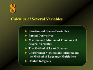
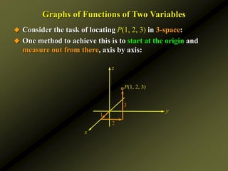
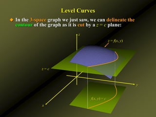
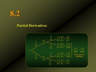
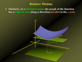
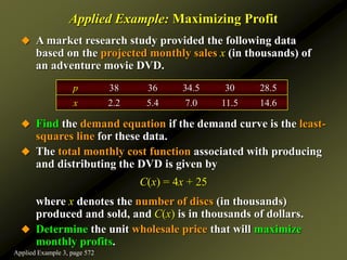
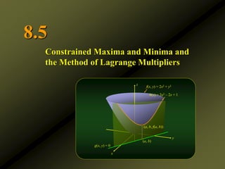
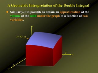
This document discusses several topics in calculus of several variables:
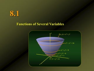
- Functions of several variables and their partial derivatives
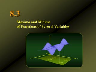
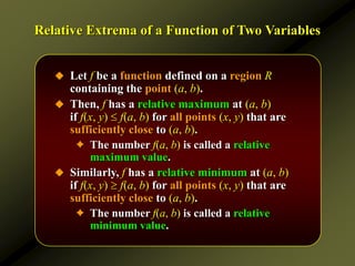
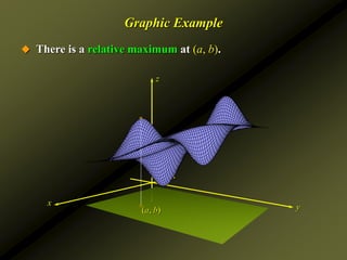
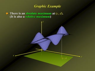
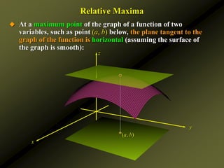
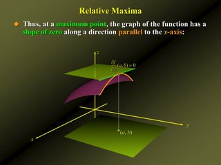
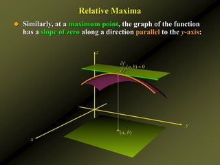
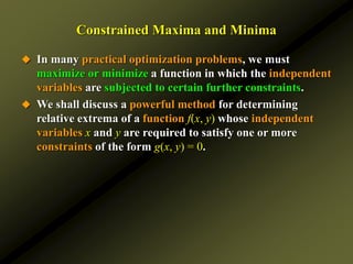
- Maxima and minima of functions of several variables
- Double integrals and constrained maxima/minima using Lagrange multipliers
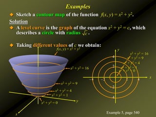
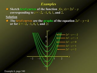
It provides examples of computing partial derivatives of functions, interpreting them geometrically, and using partial derivatives to determine rates of change. Level curves are also discussed as a way to sketch graphs of functions of two variables.


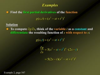

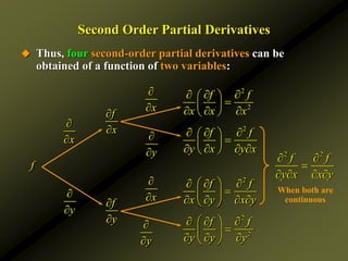

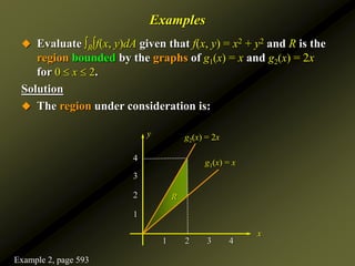
![Examples
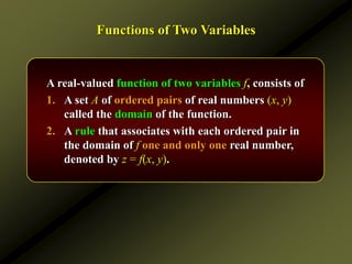
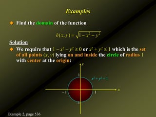
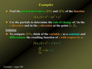
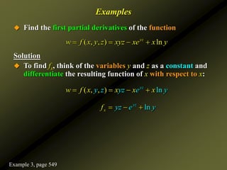
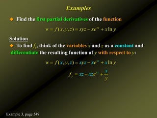
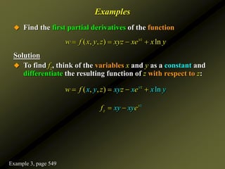
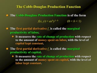
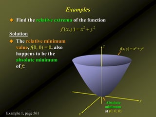
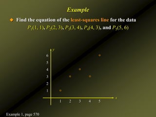
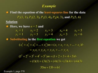
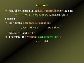
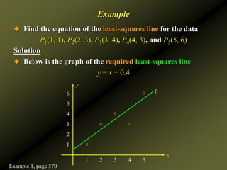
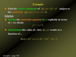
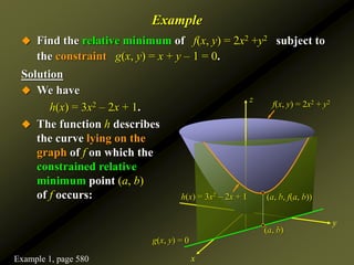
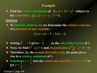
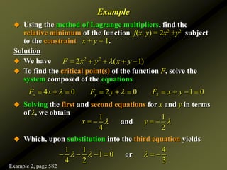
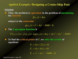
Find the relative extrema of the function
Solution
Apply the second derivative test to the critical point (0, –1):
We have D(x, y) = 48(y – 1).
In particular, D(0, –1) = 48[(–1) – 1] = – 96.
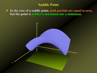
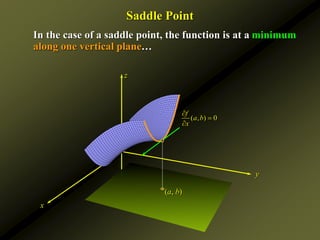
Since D(0, –1) = – 96 < 0 we conclude that f has a saddle
point at (0, –1).
The saddle point value is f (0, –1) = 22, so there is a saddle
point at (0, –1, 22).
3 2 2
( , ) 4 12 36 2
f x y y x y y
Example 3, page 562](https://image.slidesharecdn.com/pubch08-221128235749-85e3f6de/85/Calculusseveralvariables-ppt-77-320.jpg)
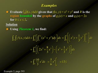
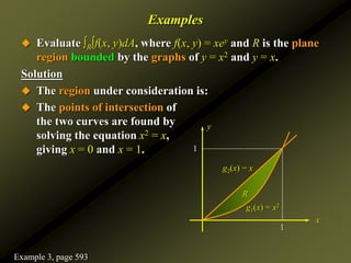
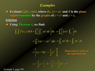
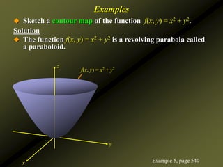
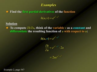
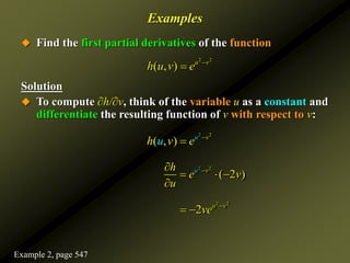
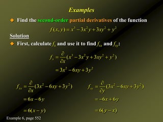
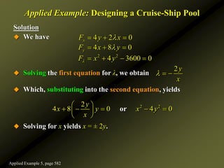
![Examples
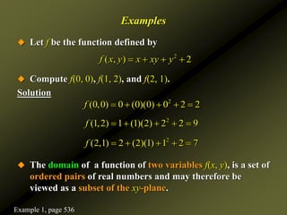
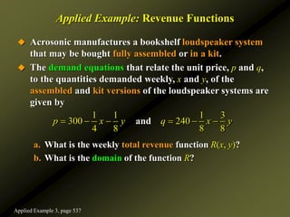
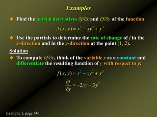
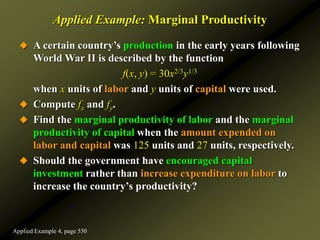
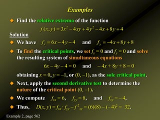
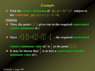
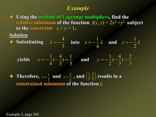
Find the relative extrema of the function
Solution
Apply the second derivative test to the critical point (0, 3):
We have D(x, y) = 48(y – 1).
In particular, D(0, 3) = 48[(3) – 1] = 96.
Since D(0, –1) = 96 > 0 and fxx (0, 3) = 2 > 0, we conclude that
f has a relative minimum at the point (0, 3).
The relative minimum value, f (0, 3) = –106, so there is a
relative minimum at (0, 3, –106).
3 2 2
( , ) 4 12 36 2
f x y y x y y
Example 3, page 562](https://image.slidesharecdn.com/pubch08-221128235749-85e3f6de/85/Calculusseveralvariables-ppt-78-320.jpg)
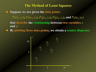
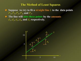
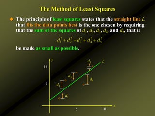
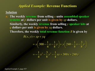
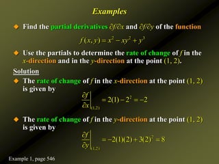
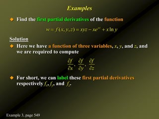
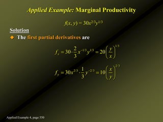
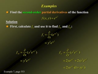
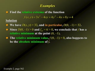
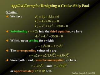
![The Method of Least Squares
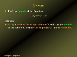
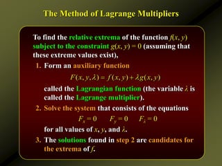
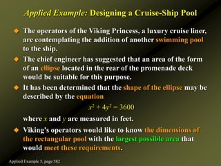
Observe that
This may be viewed as a function of two variables m and b.
Thus, the least-squares criterion is equivalent to minimizing
the function
2 2 2 2 2
1 2 3 4 5
d d d d d
2 2 2
1 1 2 2 3 3
2 2
4 4 5 5
[ ( ) ] [ ( ) ] [ ( ) ]
[ ( ) ] [ ( ) ]
f x y f x y f x y
f x y f x y
2 2 2
1 1 2 2 3 3
2 2
4 4 5 5
[ ] [ ] [ ]
[ ] [ ]
mx b y mx b y mx b y
mx b y mx b y
2 2 2
1 1 2 2 3 3
2 2
4 4 5 5
( , ) ( ) ( ) ( )
( ) ( )
f m b mx b y mx b y mx b y
mx b y mx b y
](https://image.slidesharecdn.com/pubch08-221128235749-85e3f6de/85/Calculusseveralvariables-ppt-89-320.jpg)
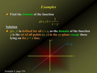
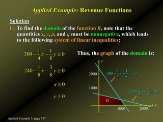
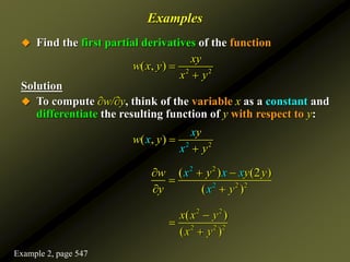
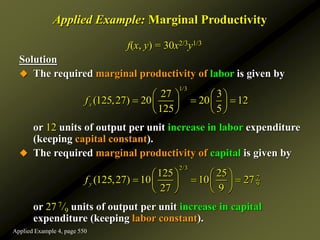
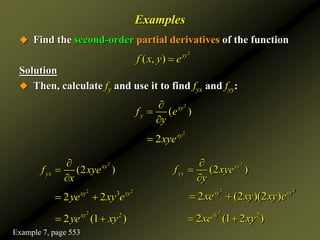
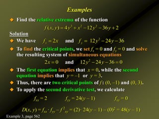
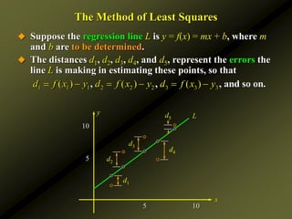
![The Method of Least Squares
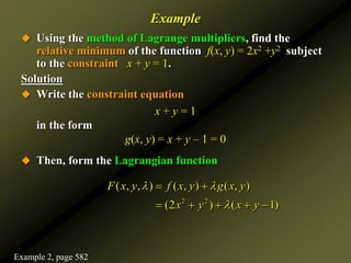
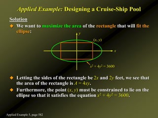
We want to minimize
We first find the partial derivative with respect to m:
1 1 1 2 2 2 3 3 3
4 4 4 5 5 5
2( ) 2( ) 2( )
2( ) 2( )
f
mx b y x mx b y x mx b y x
m
mx b y x mx b y x
2 2 2
1 1 1 1 2 2 2 2 3 3 3 3
2 2
4 4 4 4 5 5 5 5
2[
]
mx bx y x mx bx y x mx bx y x
mx bx y x mx bx y x
2 2 2 2 2
1 2 3 4 5 1 2 3 4 5
1 1 2 2 3 3 4 4 5 5
2[( ) ( )
( )]
x x x x x m x x x x x b
y x y x y x y x y x
2 2 2
1 1 2 2 3 3
2 2
4 4 5 5
( , ) ( ) ( ) ( )
( ) ( )
f m b mx b y mx b y mx b y
mx b y mx b y
](https://image.slidesharecdn.com/pubch08-221128235749-85e3f6de/85/Calculusseveralvariables-ppt-90-320.jpg)
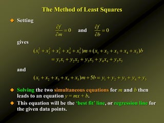
![The Method of Least Squares
We want to minimize
We now find the partial derivative with respect to b:
1 1 2 2 3 3
4 4 5 5
2( ) 2( ) 2( )
2( ) 2( )
f
mx b y mx b y mx b y
b
mx b y mx b y
1 2 3 4 5 1 2 3 4 5
2[( ) 5 ( )]
x x x x x m b y y y y y
2 2 2
1 1 2 2 3 3
2 2
4 4 5 5
( , ) ( ) ( ) ( )
( ) ( )
f m b mx b y mx b y mx b y
mx b y mx b y
](https://image.slidesharecdn.com/pubch08-221128235749-85e3f6de/85/Calculusseveralvariables-ppt-91-320.jpg)
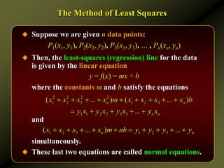

![Solution
To find the absolute maximum of P(x) over the closed
interval [0, 49.37], we compute
Since P(x) = 0 , we find that x ≈ 22.22 as the only critical
point of P.
Finally, from the table
we see that the optimal wholesale price is
or $21.99 per disc.
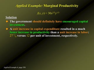
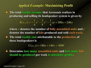
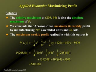
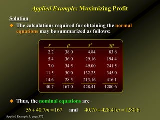
Applied Example: Maximizing Profit
( ) 1.62 35.99
P x x
x 0 22.22 49.37
P(x) –25 374.78 – 222.47
0.81(22.22) 39.99 21.99
p
Applied Example 3, page 572](https://image.slidesharecdn.com/pubch08-221128235749-85e3f6de/85/Calculusseveralvariables-ppt-103-320.jpg)
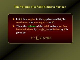
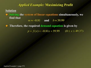
![ You may recall that we can do a Riemann sum to
approximate the area under the graph of a function of one
variable by adding the areas of the rectangles that form
below the graph resulting from small increments of x (x)
within a given interval [a, b]:
x
y
A Geometric Interpretation of the Double Integral
y= f(x)
a b
x](https://image.slidesharecdn.com/pubch08-221128235749-85e3f6de/85/Calculusseveralvariables-ppt-120-320.jpg)
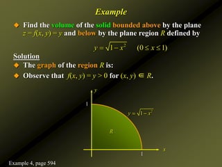
![Theorem 1
Evaluating a Double Integral Over a Plane Region
a. Suppose g1(x) and g2(x) are continuous functions on [a, b] and
the region R is defined by R = {(x, y)| g1(x) y g2(x); a x b}.
Then,
2
1
( )
( )
( , ) ( , )
b g x
R a g x
f x y dA f x y dy dx
x
y
a b
y = g1(x)
y = g2(x)
R](https://image.slidesharecdn.com/pubch08-221128235749-85e3f6de/85/Calculusseveralvariables-ppt-126-320.jpg)
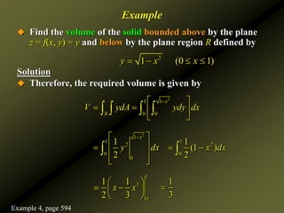
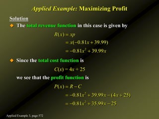
![Theorem 1
Evaluating a Double Integral Over a Plane Region
b. Suppose h1(y) and h2(y) are continuous functions on [c, d] and
the region R is defined by R = {(x, y)| h1(y) x h2(y); c y d}.
Then,
2
1
( )
( )
( , ) ( , )
d h y
R c h y
f x y dA f x y dx dy
x
y
c
d
x = h1(y) x = h2(y)
R](https://image.slidesharecdn.com/pubch08-221128235749-85e3f6de/85/Calculusseveralvariables-ppt-127-320.jpg)