Download to read offline

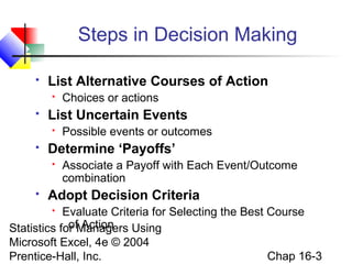
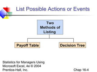
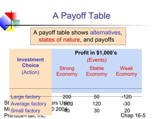
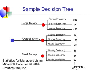
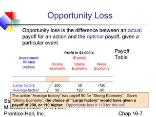
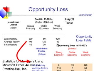
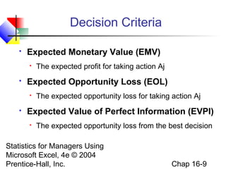
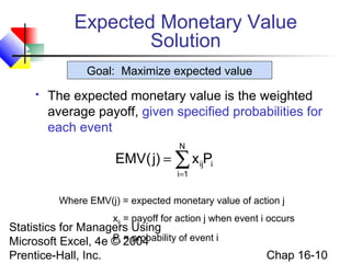
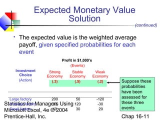
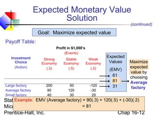
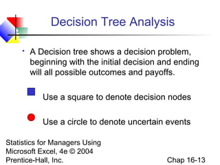
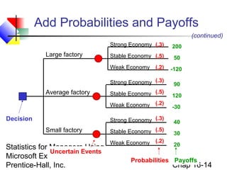
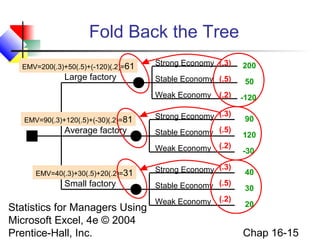
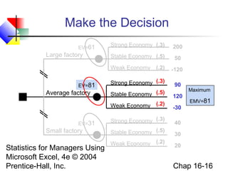
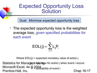
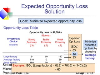
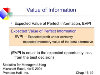
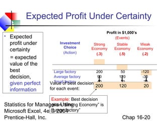
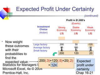
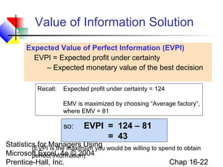
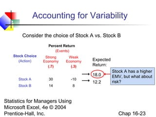
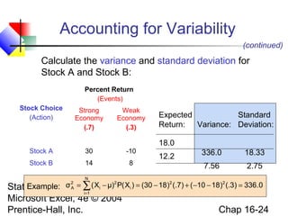
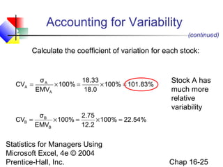
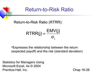
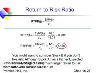
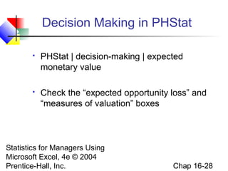
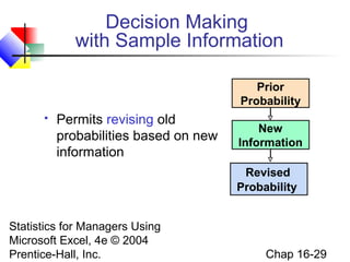
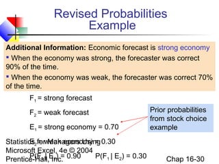
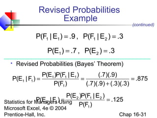
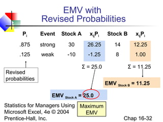
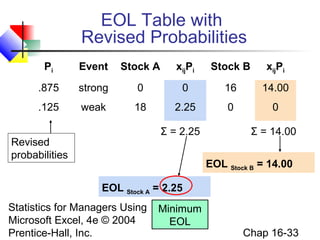
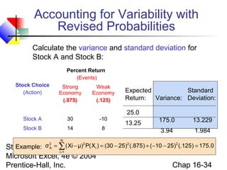
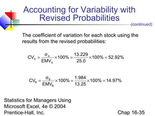
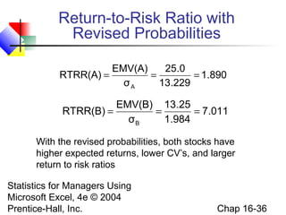
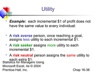
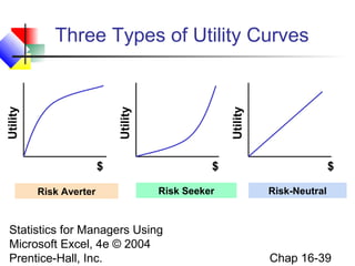

This chapter discusses decision making under uncertainty. It describes the basic steps in decision making as listing alternative actions, uncertain events, determining payoffs, and adopting decision criteria. It introduces payoff tables and decision trees as methods to display this information. Expected monetary value and expected opportunity loss are presented as decision criteria that aim to maximize expected payoff or minimize expected loss. The value of perfect information is defined as the expected gain from knowing the outcome with certainty compared to the best action under uncertainty. Finally, it discusses how to account for risk by considering the variability of payoffs through measures like variance and standard deviation.


![[DSC Europe 25] Elena Menshikova - AI-Powered Operational Excellence: Revolut...](https://cdn.slidesharecdn.com/ss_thumbnails/es6nholbqy3zaao2c2yd-2-elena-menshikova-data-ai-in-decision-making-260115093812-4fba8b38-thumbnail.jpg?width=640&height=640&fit=bounds)

![[DSC Europe 25] Andrzej Kowalczyk - AI - how to start small and grow in the f...](https://cdn.slidesharecdn.com/ss_thumbnails/oy1zmo94qv6vpcqjvno2-andrzej-kowalczyk-ai-how-to-start-small-and-grow-in-the-future-1-260119121559-cf093b23-thumbnail.jpg?width=640&height=640&fit=bounds)


![[DSC Europe 25] Ivan Lukovic & Marija Djukic - From Data to Value: Why Maturi...](https://cdn.slidesharecdn.com/ss_thumbnails/ahrfps8xr6knowwhacxh-1-ivan-marija-dsc-2025-ld-v1-presentation-260115093812-be21adfc-thumbnail.jpg?width=640&height=640&fit=bounds)

![[DSC Europe 25] Bojan Djuricic - Predictive Design Process.pdf](https://cdn.slidesharecdn.com/ss_thumbnails/5awdrbedqdek3gqu2ezy-4-the-predictive-design-bojan-djuricic-260120105856-6c399e9b-thumbnail.jpg?width=640&height=640&fit=bounds)


