This document discusses foundational concepts in probability and probability distributions that are important for teaching basic statistics. It introduces key terms like random experiment, sample space, event, probability, random variable, and different probability distributions including binomial and normal. Concepts are explained through examples like rolling dice, drawing cards from a deck, and the probabilities of related outcomes. The goal is to equip readers with a basic understanding of probability theory needed to assess estimates from sample data and determine adequate sample sizes.
Session 2.2
TEACHING BASICSTATISTICS
Motivation for Studying Chance
Sample Statistic Estimates Population Parameter
e.g. Sample Mean X = 50 estimates Population Mean m
Questions:
1. How do we assess the reliability of our estimate?
2. What is an adequate sample size? [ We would expect a
large sample to give better estimates. Large samples
more costly.]
3.
Session 2.3
TEACHING BASICSTATISTICS
An Approach to Solve the Questions
If sample was chosen through
chance processes, we have to
understand the notion of
probability and sampling
distribution.
4.
Session 2.4
TEACHING BASICSTATISTICS
To introduce probability….
Random experiment
Sample space
Event as subset of sample
space
Likelihood of an event to occur
- probability of an event
5.
Session 2.5
TEACHING BASICSTATISTICS
Features of a Random Experiment
All outcomes are known in
advance.
The outcome of any one
trial is unpredictable.
Trials are repeatable under
identical conditions.
6.
Session 2.6
TEACHING BASICSTATISTICS
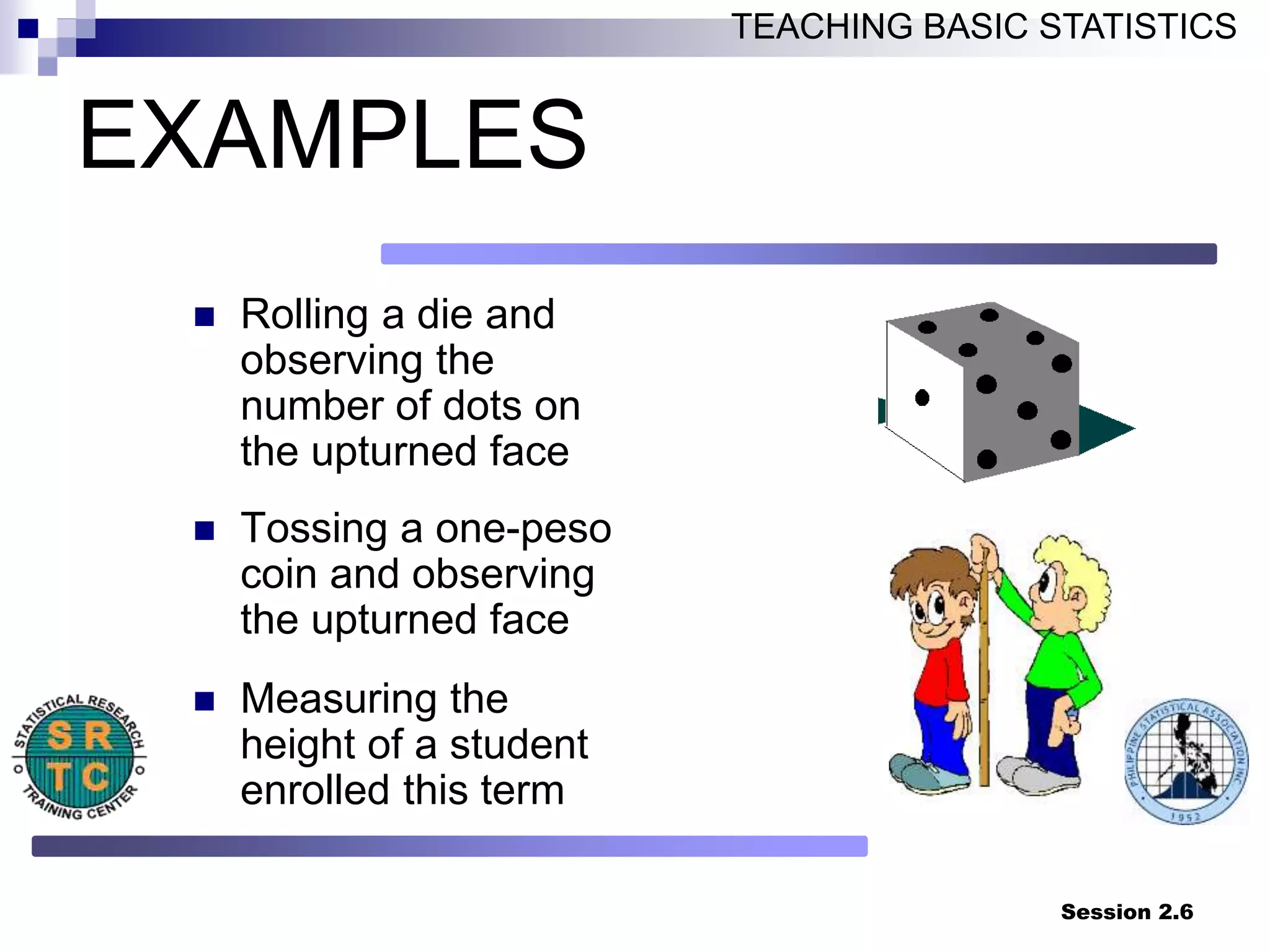
EXAMPLES
Rolling a die and
observing the
number of dots on
the upturned face
Tossing a one-peso
coin and observing
the upturned face
Measuring the
height of a student
enrolled this term
7.
Session 2.7
TEACHING BASICSTATISTICS
SAMPLE SPACE
It is a set such that each element
denotes an outcome of a random
experiment.
Any performance of the
experiment results in an outcome
that corresponds to exactly one
and only one element.
It is usually denoted by S.
8.
Session 2.8
TEACHING BASICSTATISTICS
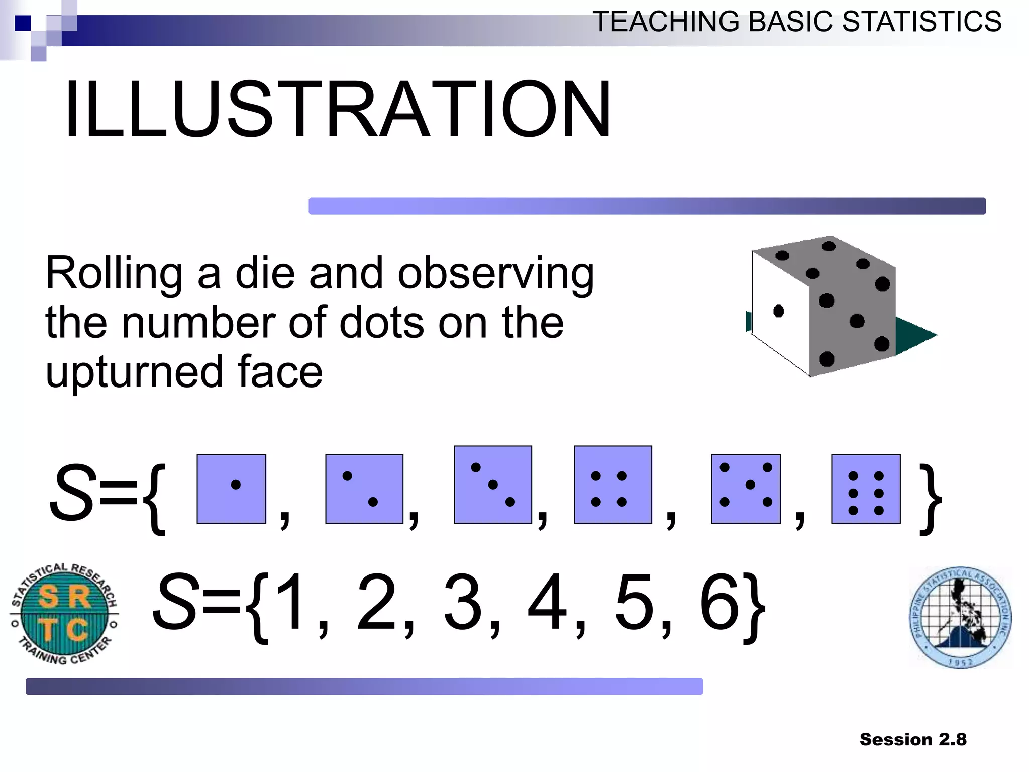
ILLUSTRATION
Rolling a die and observing
the number of dots on the
upturned face
S={ , , , , , }
S={1, 2, 3, 4, 5, 6}
9.
Session 2.9
TEACHING BASICSTATISTICS
EVENT
A subset of the sample space
Usually denoted by capital letters like
E, A or B
Observance of the elements of the
subset implies the occurrence of the
event
Can either be classified as simple or
compound event
10.
Session 2.10
TEACHING BASICSTATISTICS
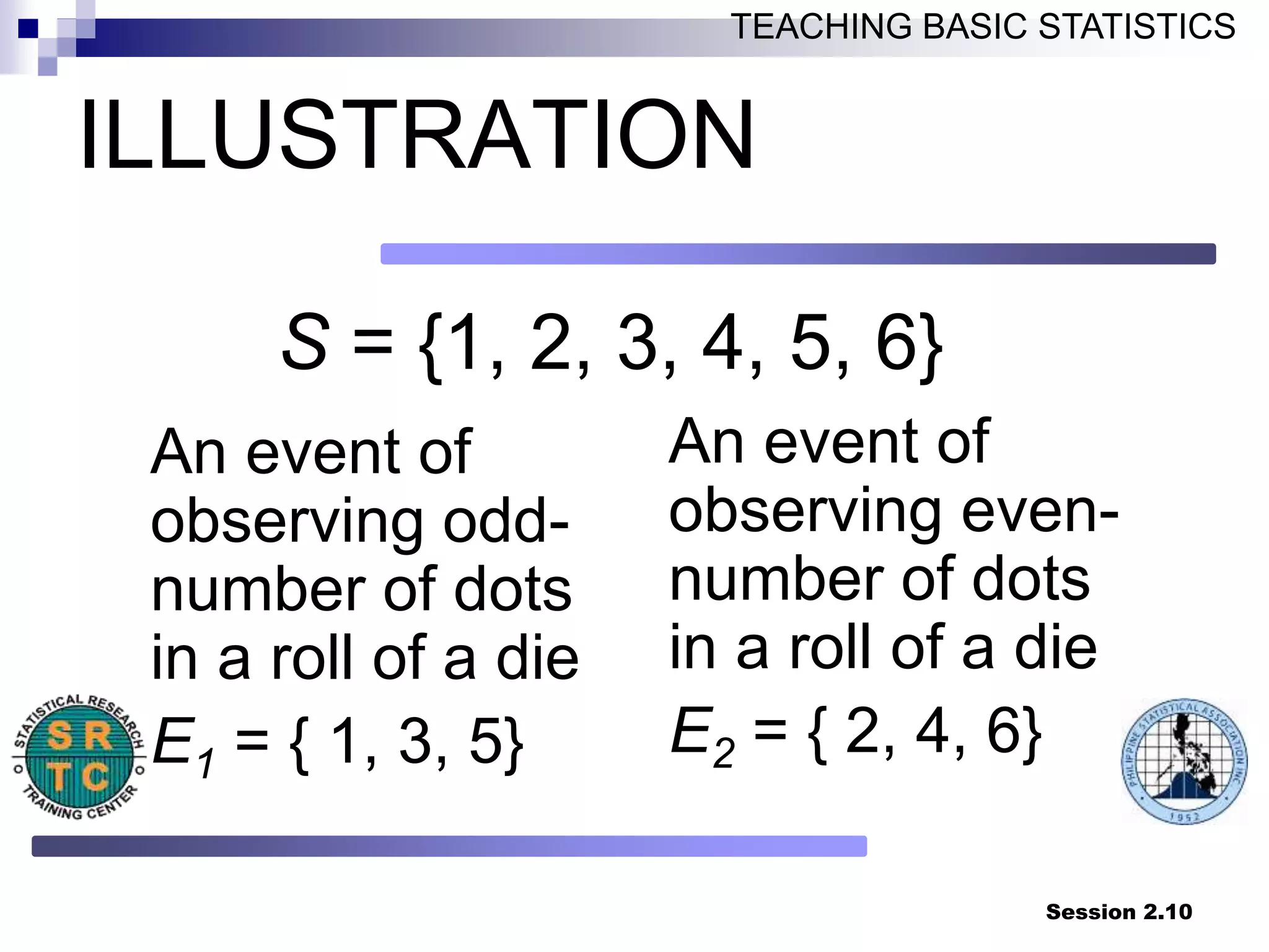
ILLUSTRATION
S = {1, 2, 3, 4, 5, 6}
An event of
observing odd-
number of dots
in a roll of a die
E1 = { 1, 3, 5}
An event of
observing even-
number of dots
in a roll of a die
E2 = { 2, 4, 6}
11.
Session 2.11
TEACHING BASICSTATISTICS
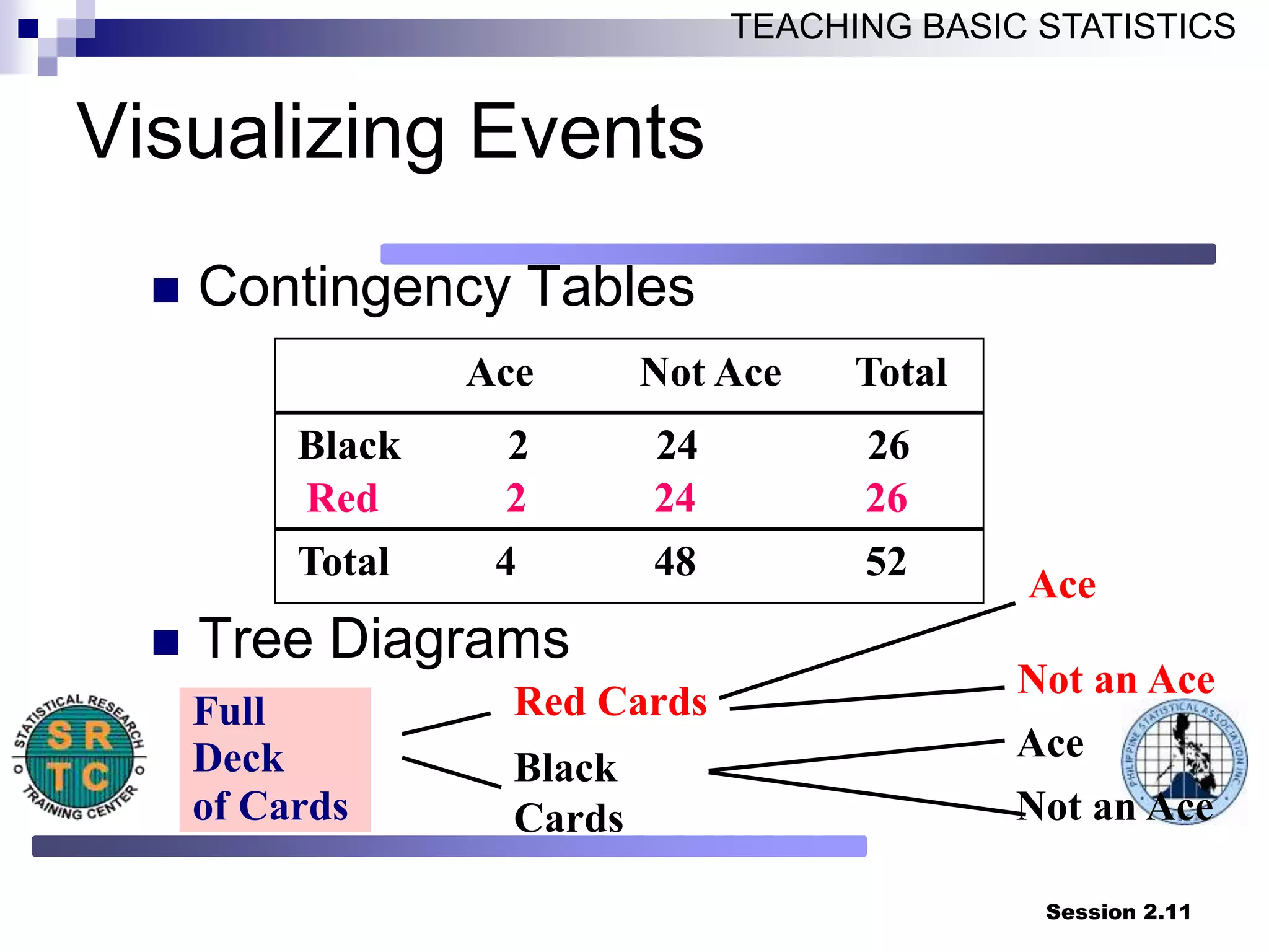
Visualizing Events
Contingency Tables
Tree Diagrams
Red 2 24 26
Black 2 24 26
Total 4 48 52
Ace Not Ace Total
Full
Deck
of Cards
Red Cards
Black
Cards
Not an Ace
Ace
Ace
Not an Ace
12.
Session 2.12
TEACHING BASICSTATISTICS
Mutually Exclusive Events
Two events are mutually exclusive if
one and only one of them can occur at a
time.
Example:
Coin toss: either a head or a tail, but not
both. The events head and tail are
mutually exclusive.
13.
Session 2.13
TEACHING BASICSTATISTICS
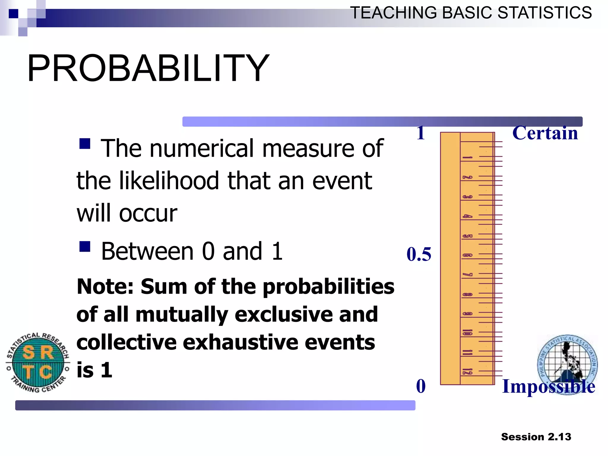
The numerical measure of
the likelihood that an event
will occur
Between 0 and 1
Note: Sum of the probabilities
of all mutually exclusive and
collective exhaustive events
is 1
Certain
Impossible
0.5
1
0
PROBABILITY
14.
Session 2.14
TEACHING BASICSTATISTICS
Assigning Probabilities
Subjective
confident student views chances of passing
a course to be near 100 %
Logical
symmetry/equally likely: coin, dice, cards etc.
(A PRIORI assignment)
Empirical
chances of rain 75 % since it rained 15 out of
past 20 days (A POSTERIORI)
15.
Session 2.15
TEACHING BASICSTATISTICS
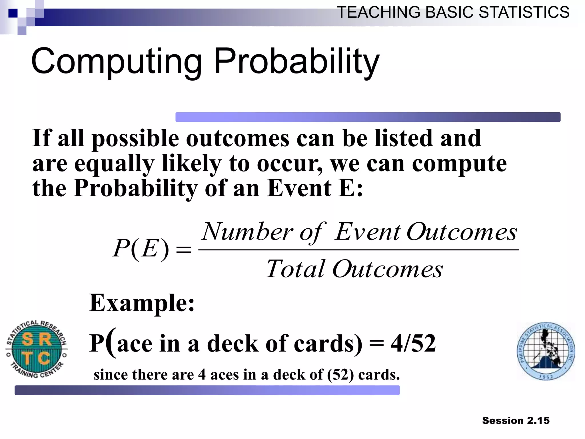
If all possible outcomes can be listed and
are equally likely to occur, we can compute
the Probability of an Event E:
Outcomes
Total
Outcomes
Event
of
Number
E
P
)
(
Example:
P(ace in a deck of cards) = 4/52
since there are 4 aces in a deck of (52) cards.
Computing Probability
16.
Session 2.16
TEACHING BASICSTATISTICS
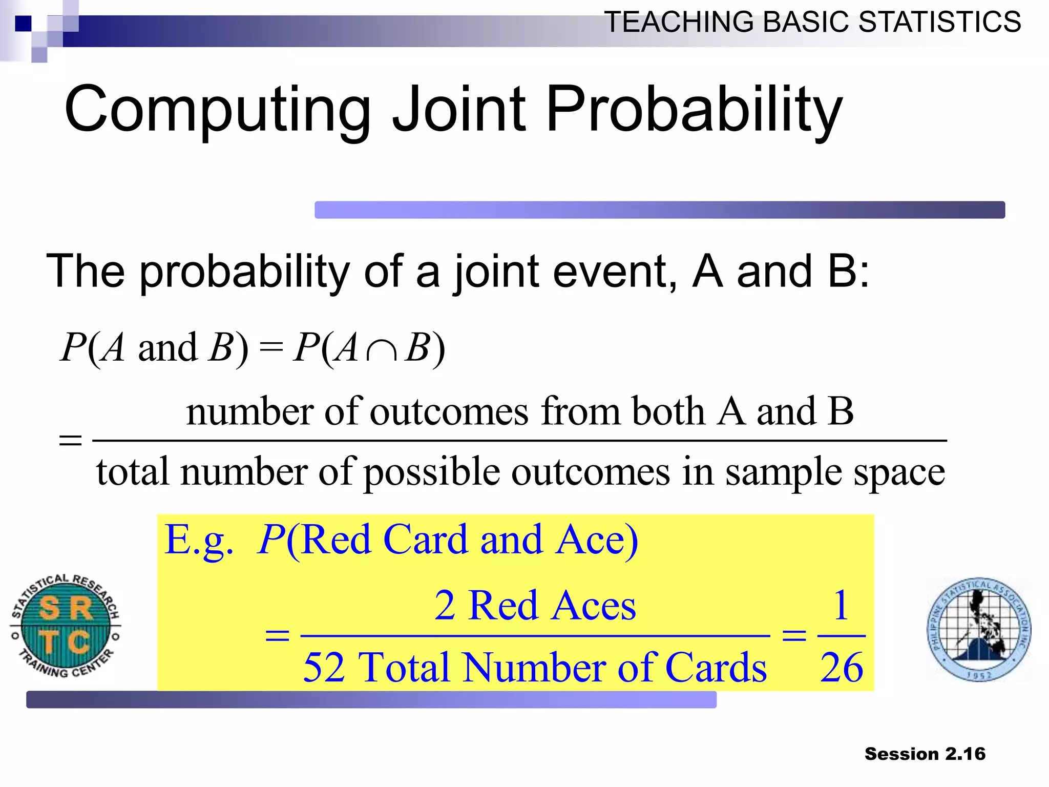
Computing Joint Probability
The probability of a joint event, A and B:
( and ) = ( )
number of outcomes from both A and B
total number of possible outcomes in sample space
P A B P A B
E.g. (Red Card and Ace)
2 Red Aces 1
52 Total Number of Cards 26
P
17.
Session 2.17
TEACHING BASICSTATISTICS
Rules on Probability
Property 1. The probability of an
event E is any number between 0
and 1 inclusive.
Property 2. The sum of the
probabilities of a set of mutually
exclusive events is 1.
18.
Session 2.18
TEACHING BASICSTATISTICS
Rules on Probability
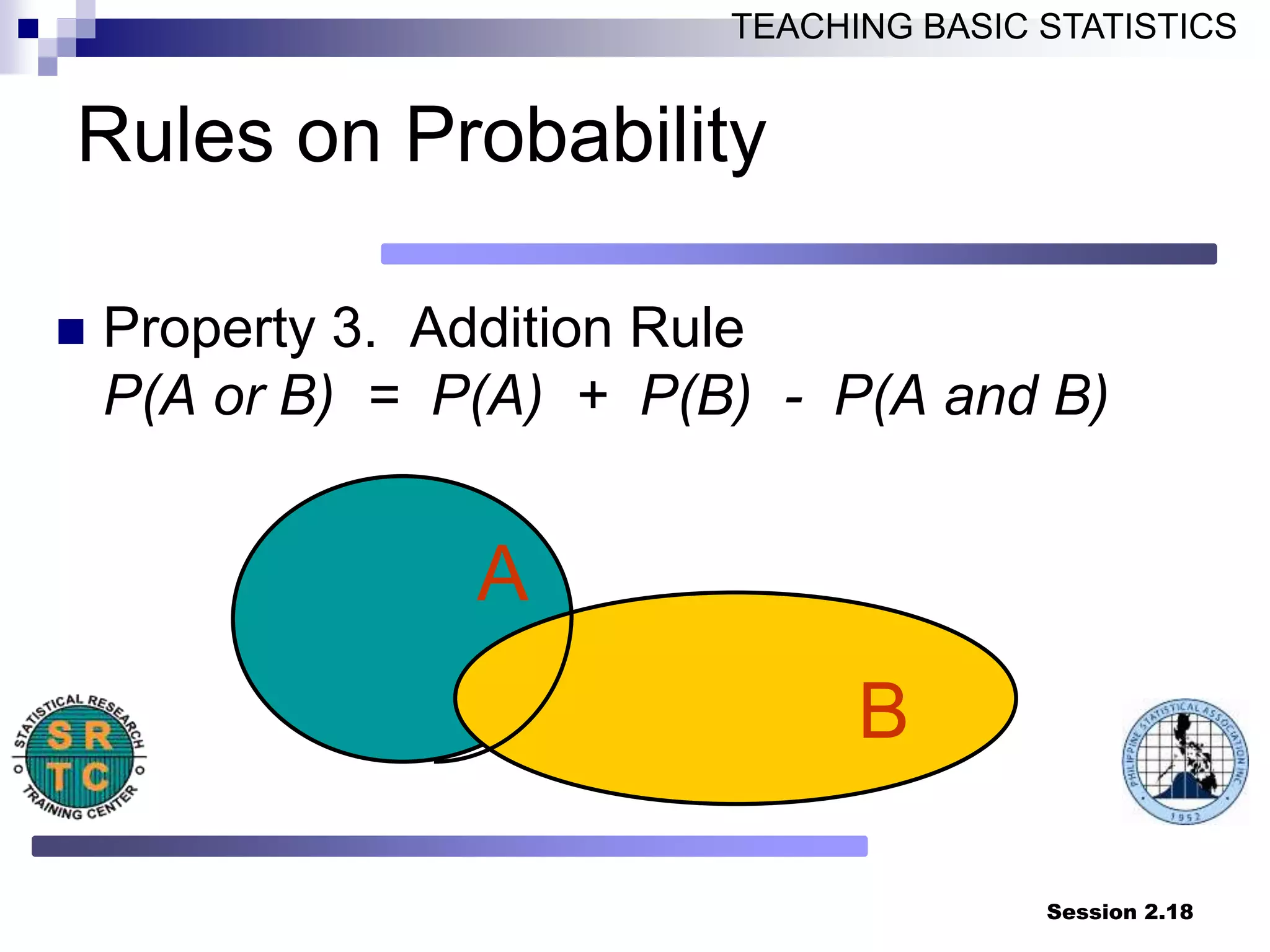
Property 3. Addition Rule
P(A or B) = P(A) + P(B) - P(A and B)
A
B
19.
Session 2.19
TEACHING BASICSTATISTICS
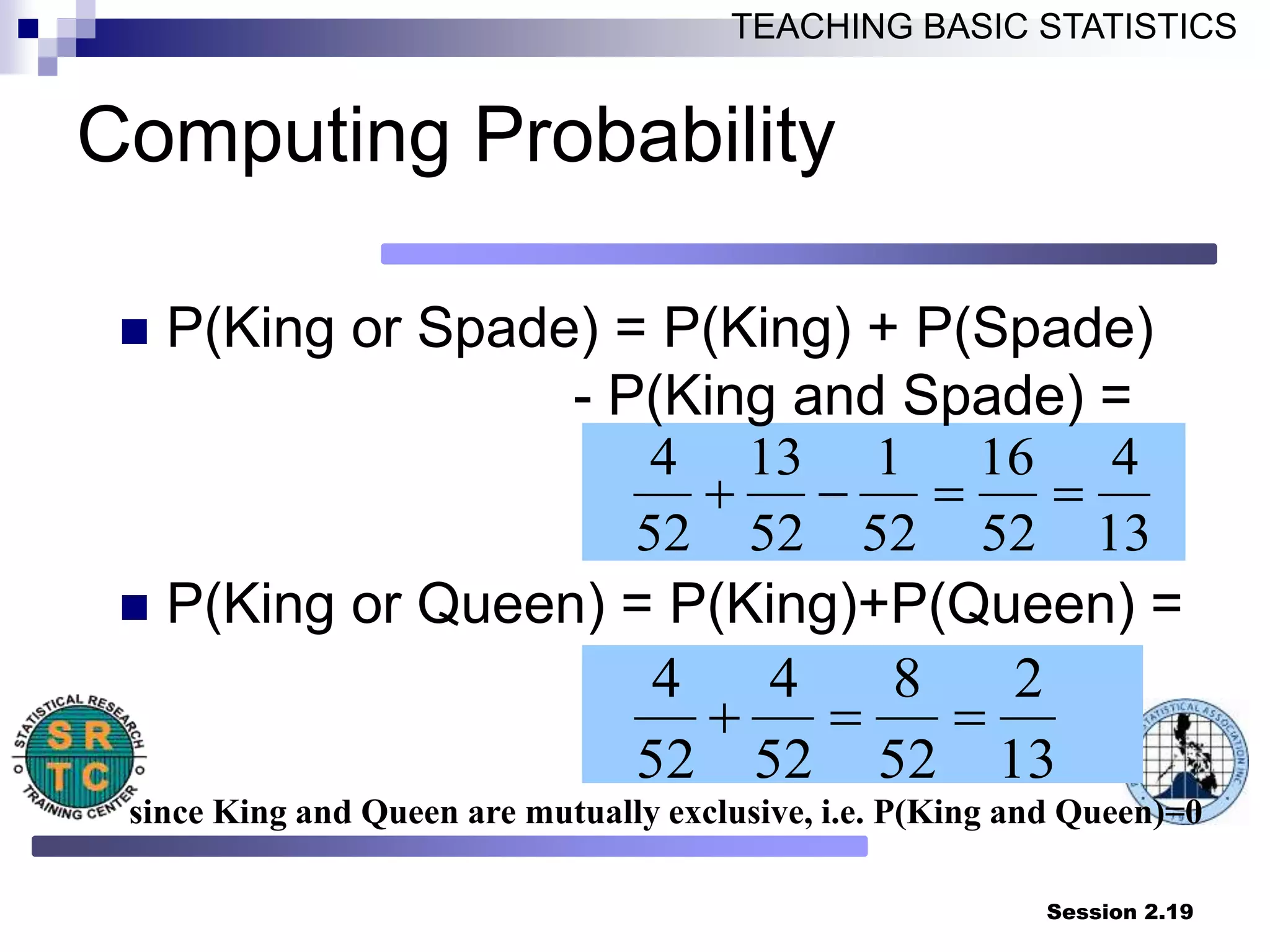
Computing Probability
P(King or Spade) = P(King) + P(Spade)
- P(King and Spade) =
P(King or Queen) = P(King)+P(Queen) =
13
4
52
16
52
1
52
13
52
4
13
2
52
8
52
4
52
4
since King and Queen are mutually exclusive, i.e. P(King and Queen)=0
20.
Session 2.20
TEACHING BASICSTATISTICS
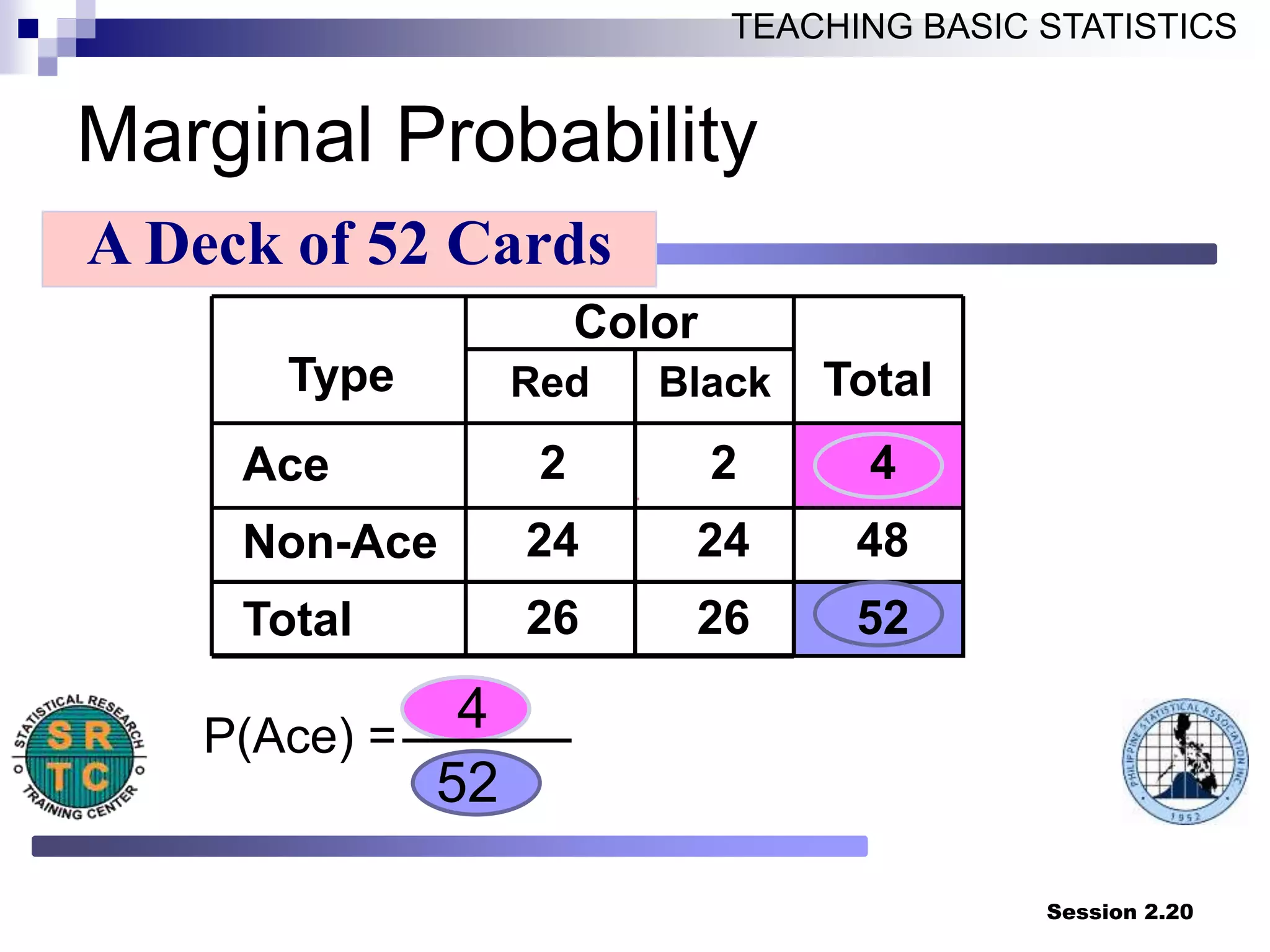
Marginal Probability
Black
Color
Type Red Total
Ace 2 2 4
Non-Ace 24 24 48
Total 26 26 52
P(Ace) =
4
52
A Deck of 52 Cards
21.
Session 2.21
TEACHING BASICSTATISTICS
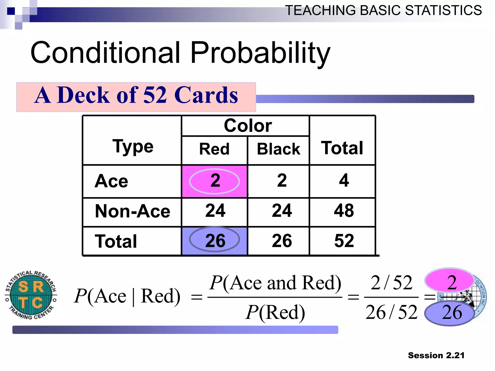
Conditional Probability
Black
Color
Type Red Total
Ace 2 2 4
Non-Ace 24 24 48
Total 26 26 52
(Ace and Red) 2/52 2
(Ace | Red)
(Red) 26/52 26
P
P
P
A Deck of 52 Cards
22.
Session 2.22
TEACHING BASICSTATISTICS
Joint Probability
Multiplication Rule:
The chance that two events will
occur is the chance that the first
event will occur multiplied by the
chance of the second event (given
that the first has happened)
23.
Session 2.23
TEACHING BASICSTATISTICS
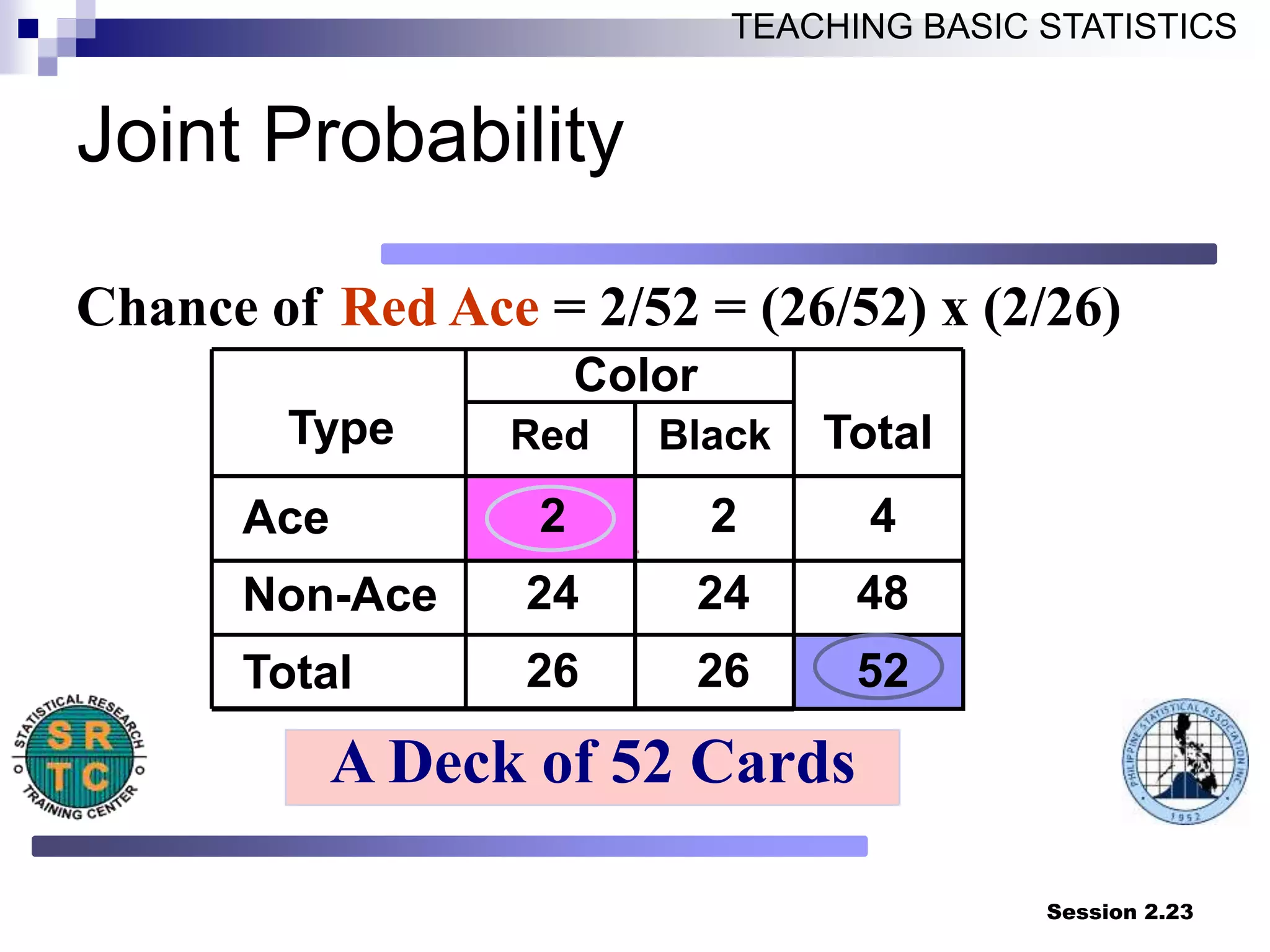
Joint Probability
A Deck of 52 Cards
Chance of Red Ace = 2/52 = (26/52) x (2/26)
Black
Color
Type Red Total
Ace 2 2 4
Non-Ace 24 24 48
Total 26 26 52
24.
Session 2.24
TEACHING BASICSTATISTICS
UNEQUALLY LIKELY OUTCOME
ASSUMPTION
The outcomes have different
likelihood to occur.
The probability of an event E is
then computed as the sum of the
probabilities of the outcomes
found in the event E, that is,
P[E] = sum of p{e}
where e is an element of event E.
25.
Session 2.25
TEACHING BASICSTATISTICS
ILLUSTRATION
S = {1, 2, 3, 4, 5, 6}
Assuming that the probability of each of the
outcomes 1,2, and 3 is 1/12 while each of the
outcomes 4, 5 and 6 has likelihood to occur
equal to 1/4.
The probability of an event of observing odd-
number of dots in a roll of a die is P[E1] = sum
of p{1}, p{3} and p{5} = 1/12 + 1/12 + 1/4 =
5/12.
26.
Session 2.26
TEACHING BASICSTATISTICS
A POSTERIORI APPROACH
The random experiment has to
be performed and the event of
interest is observed.
The probability of the event is
the relative frequency of the
occurrence of such event.
27.
Session 2.27
TEACHING BASICSTATISTICS
ILLUSTRATION
Suppose the experiment was done
for 100 times and it was observed
that an odd-number of dots occurred
60 times and even-number of dots
occurred 40 times.
The probability of an event of
observing odd-number of dots in a
roll of a die is the relative frequency
of the event or P[E1] = 60/100 = 0.6
28.
Session 2.28
TEACHING BASICSTATISTICS
Random Variable
Defined on a random experiment
A rule or a function that maps
each element of the sample to
one and only one real number
The mapping produces mutually
exclusive partitioning on the set
of real numbers
29.
Session 2.29
TEACHING BASICSTATISTICS
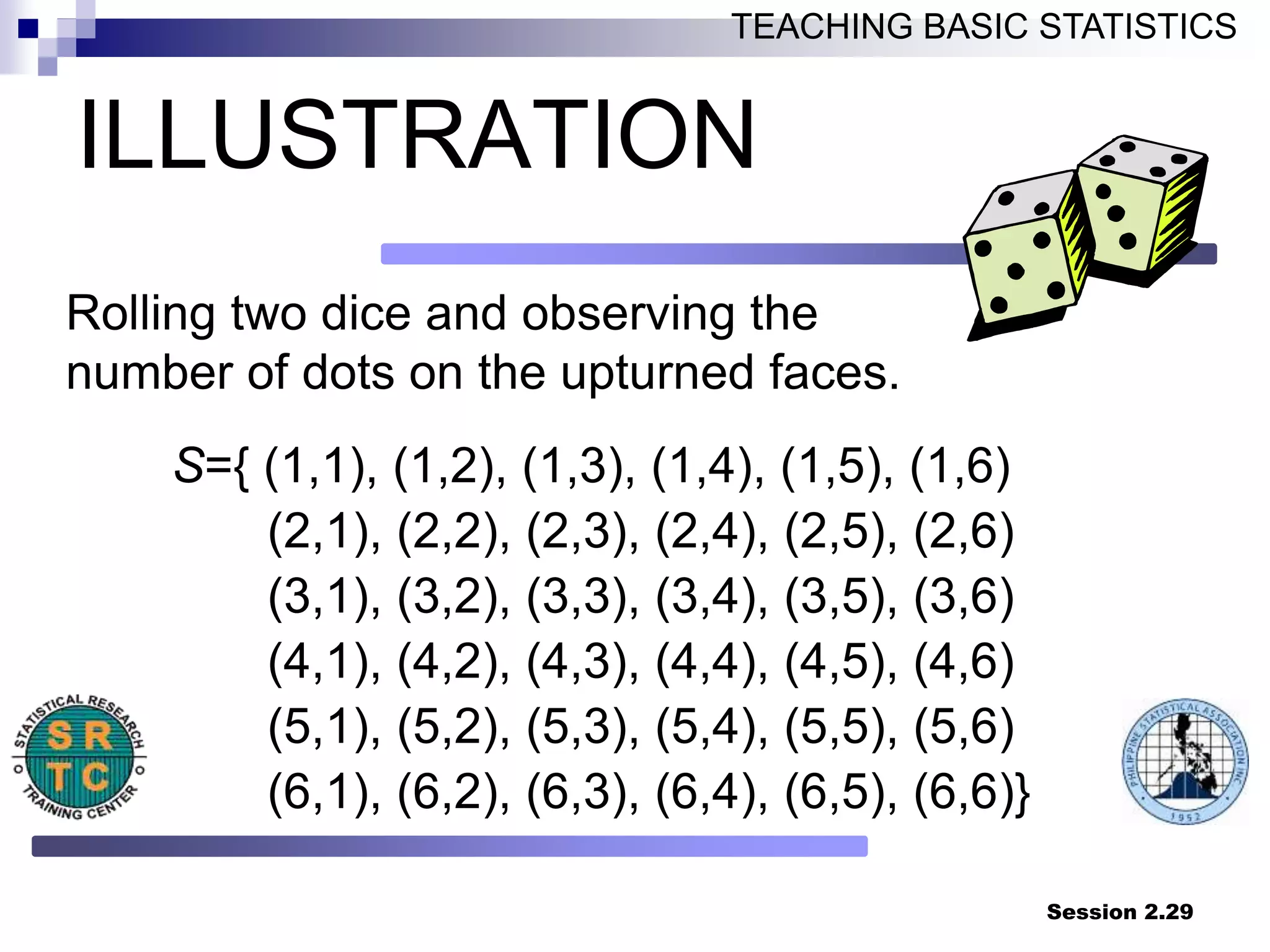
ILLUSTRATION
Rolling two dice and observing the
number of dots on the upturned faces.
S={ (1,1), (1,2), (1,3), (1,4), (1,5), (1,6)
(2,1), (2,2), (2,3), (2,4), (2,5), (2,6)
(3,1), (3,2), (3,3), (3,4), (3,5), (3,6)
(4,1), (4,2), (4,3), (4,4), (4,5), (4,6)
(5,1), (5,2), (5,3), (5,4), (5,5), (5,6)
(6,1), (6,2), (6,3), (6,4), (6,5), (6,6)}
30.
Session 2.30
TEACHING BASICSTATISTICS
ILLUSTRATION
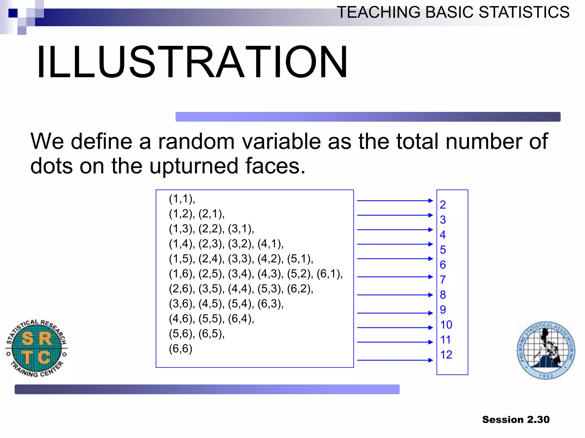
We define a random variable as the total number of
dots on the upturned faces.
2
3
4
5
6
7
8
9
10
11
12
(1,1),
(1,2), (2,1),
(1,3), (2,2), (3,1),
(1,4), (2,3), (3,2), (4,1),
(1,5), (2,4), (3,3), (4,2), (5,1),
(1,6), (2,5), (3,4), (4,3), (5,2), (6,1),
(2,6), (3,5), (4,4), (5,3), (6,2),
(3,6), (4,5), (5,4), (6,3),
(4,6), (5,5), (6,4),
(5,6), (6,5),
(6,6)
31.
Session 2.31
TEACHING BASICSTATISTICS
ILLUSTRATION
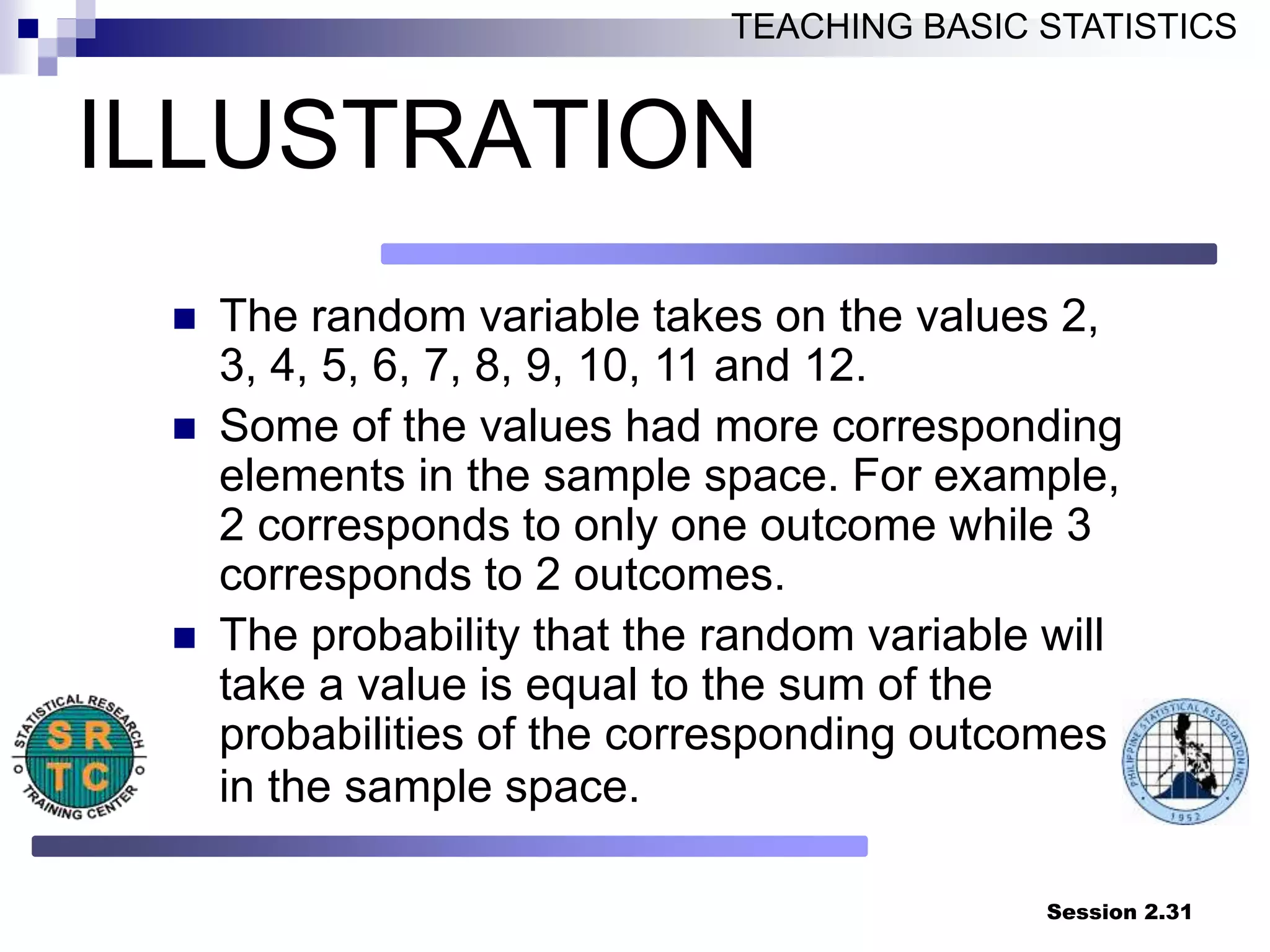
The random variable takes on the values 2,
3, 4, 5, 6, 7, 8, 9, 10, 11 and 12.
Some of the values had more corresponding
elements in the sample space. For example,
2 corresponds to only one outcome while 3
corresponds to 2 outcomes.
The probability that the random variable will
take a value is equal to the sum of the
probabilities of the corresponding outcomes
in the sample space.
32.
Session 2.32
TEACHING BASICSTATISTICS
ILLUSTRATION
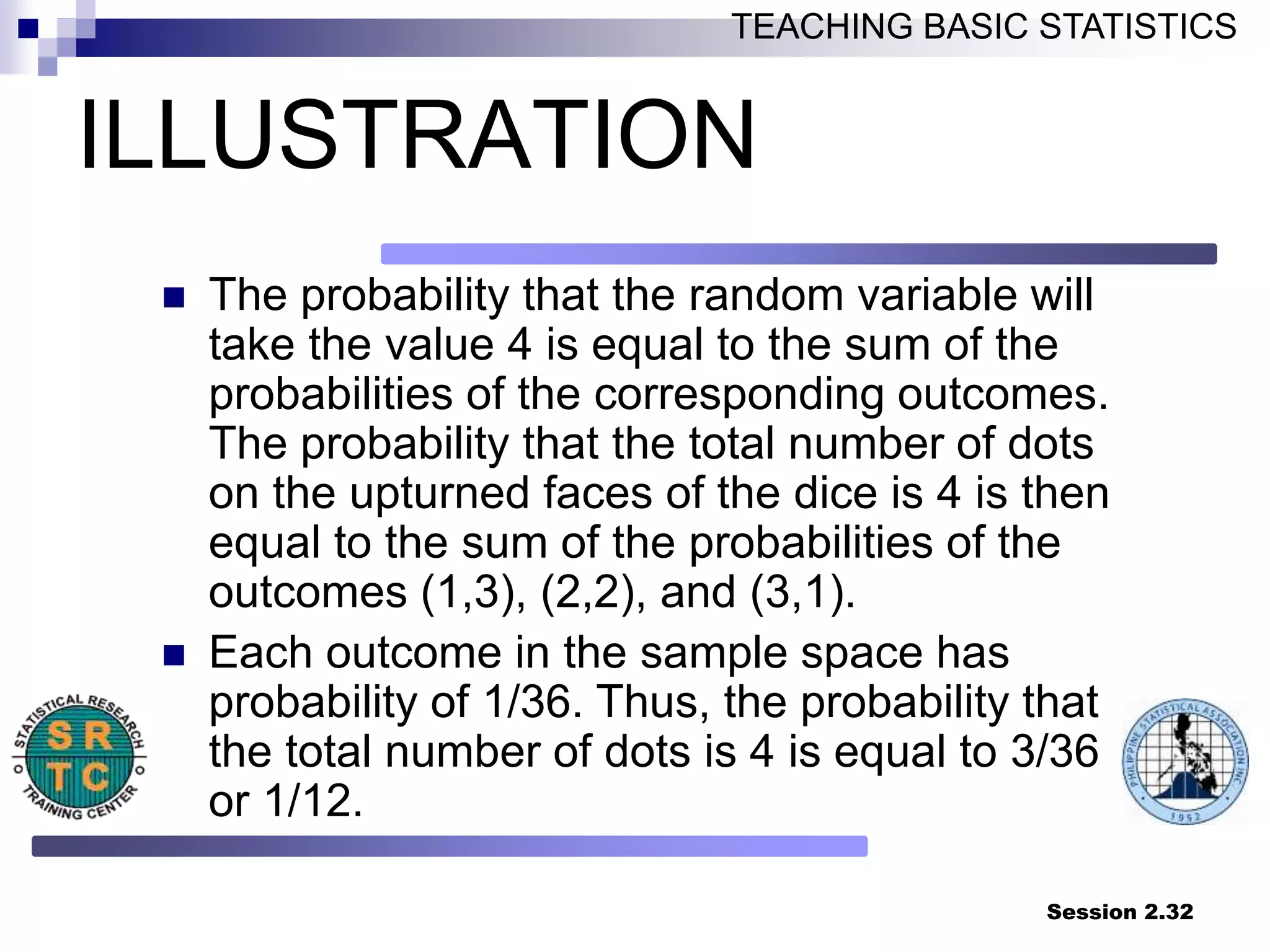
The probability that the random variable will
take the value 4 is equal to the sum of the
probabilities of the corresponding outcomes.
The probability that the total number of dots
on the upturned faces of the dice is 4 is then
equal to the sum of the probabilities of the
outcomes (1,3), (2,2), and (3,1).
Each outcome in the sample space has
probability of 1/36. Thus, the probability that
the total number of dots is 4 is equal to 3/36
or 1/12.
33.
Session 2.33
TEACHING BASICSTATISTICS
PROBABILITY DISTRIBUTION
A table or a curve or a function
that presents the possible values
of the random variable and its
corresponding probabilities.
Some random variables are
better presented as a table while
others as a function or as a
curve or graph.
34.
Session 2.34
TEACHING BASICSTATISTICS
ILLUSTRATION
The probability distribution of the random variable, X defined
as the total number of dots on the upturned faces in a roll of
two dice, is presented as a table below:
X 2 3 4 5 6 7 8 9 10 11 12
P[X=x] 1/36 2/36 3/36 4/36 5/36 6/36 5/36 4/36 3/36 2/36 1/36
0.00
0.05
0.10
0.15
0.20
2 3 4 5 6 7 8 9 10 11 12
X = Total Number of Dots on the Upturned faces
35.
Session 2.35
TEACHING BASICSTATISTICS
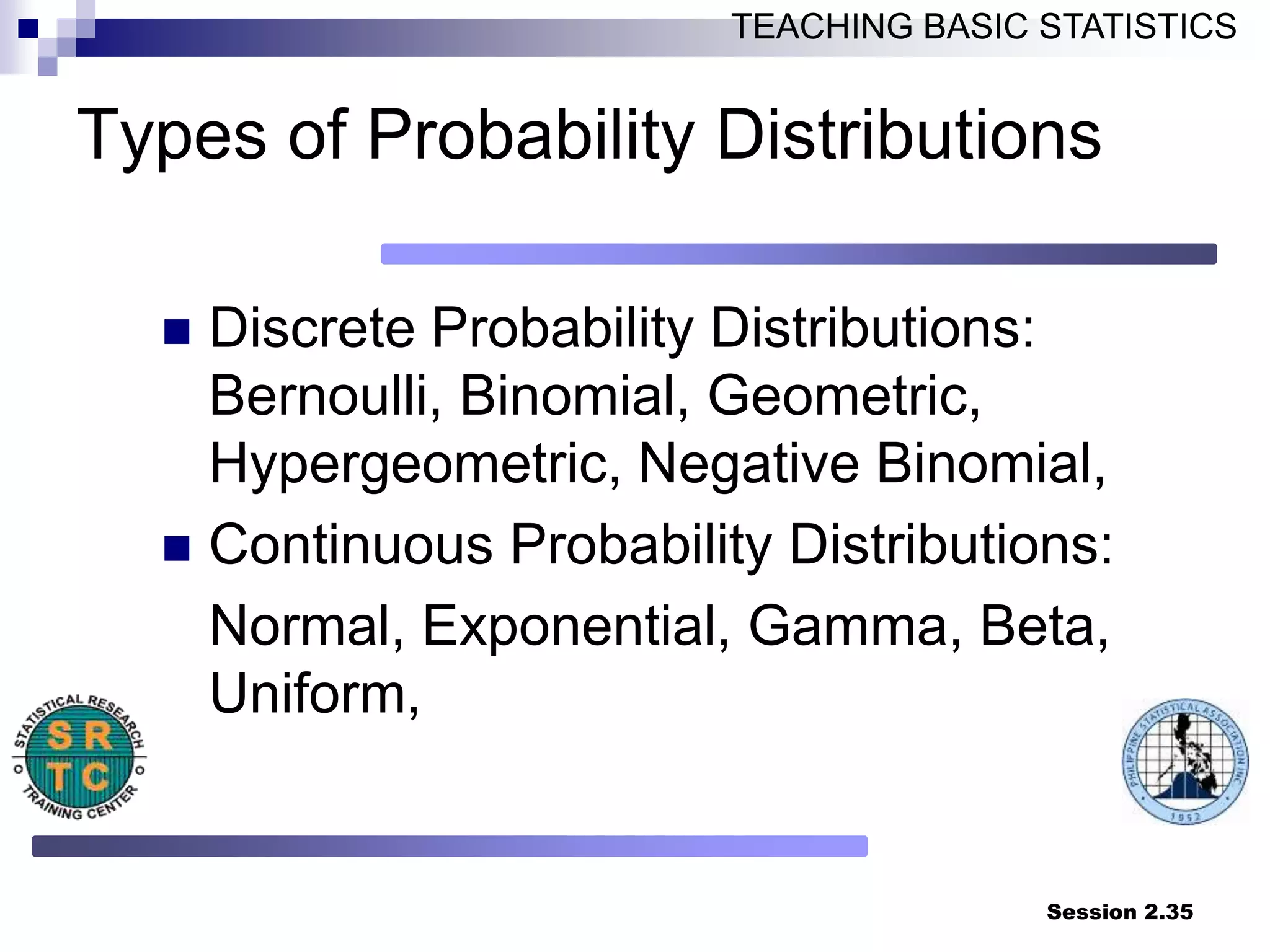
Types of Probability Distributions
Discrete Probability Distributions:
Bernoulli, Binomial, Geometric,
Hypergeometric, Negative Binomial,
Continuous Probability Distributions:
Normal, Exponential, Gamma, Beta,
Uniform,
36.
Session 2.36
TEACHING BASICSTATISTICS
Bernoulli Probability Distribution
Named after Bernoulli
Discrete random variable with
only two possible values; 0 and 1
The value 1 represents success
while the value 0 represents
failure
The parameter p is the probability
of success.
37.
Session 2.37
TEACHING BASICSTATISTICS
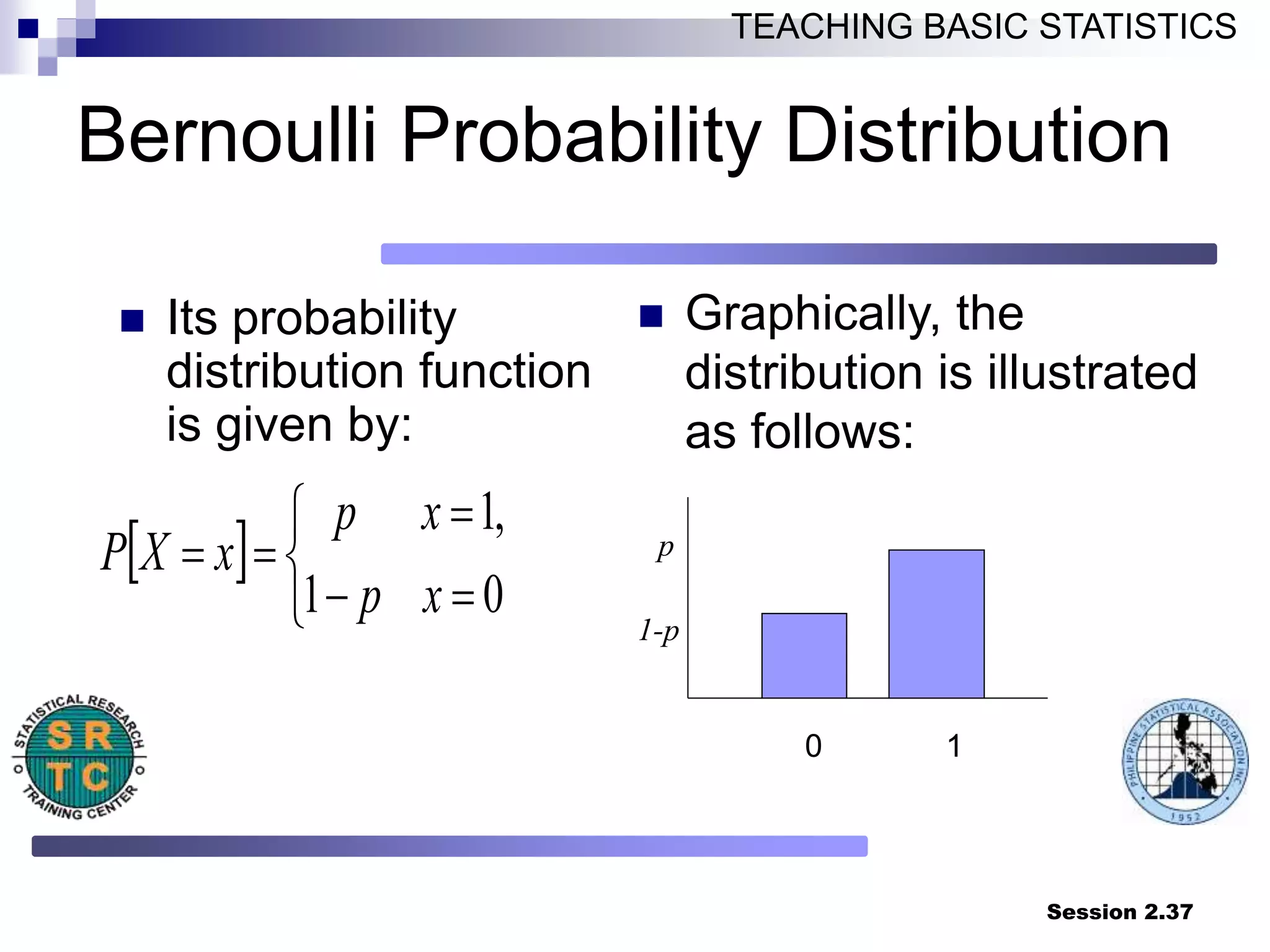
Bernoulli Probability Distribution
Its probability
distribution function
is given by:
Graphically, the
distribution is illustrated
as follows:
0
1
,
1
x
p
x
p
x
X
P
0 1
p
1-p
38.
Session 2.38
TEACHING BASICSTATISTICS
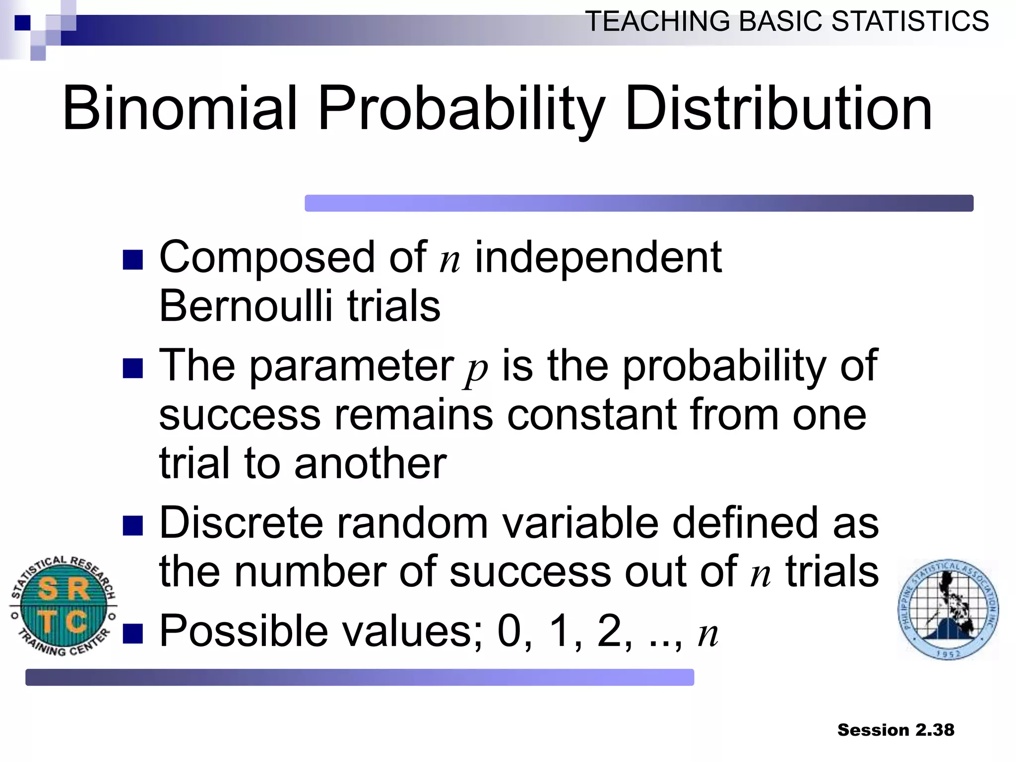
Binomial Probability Distribution
Composed of n independent
Bernoulli trials
The parameter p is the probability of
success remains constant from one
trial to another
Discrete random variable defined as
the number of success out of n trials
Possible values; 0, 1, 2, .., n
39.
Session 2.39
TEACHING BASICSTATISTICS
Binomial Probability Distribution
Its probability
distribution function is
given by:
Graphically, the
distribution is illustrated
as follows:
n
x
p
p
x
n
x
X
P
x
n
x
2,
,
1
,
0
,
1
0 1 2 …. n
and the function is
undefined elsewhere.
40.
Session 2.40
TEACHING BASICSTATISTICS
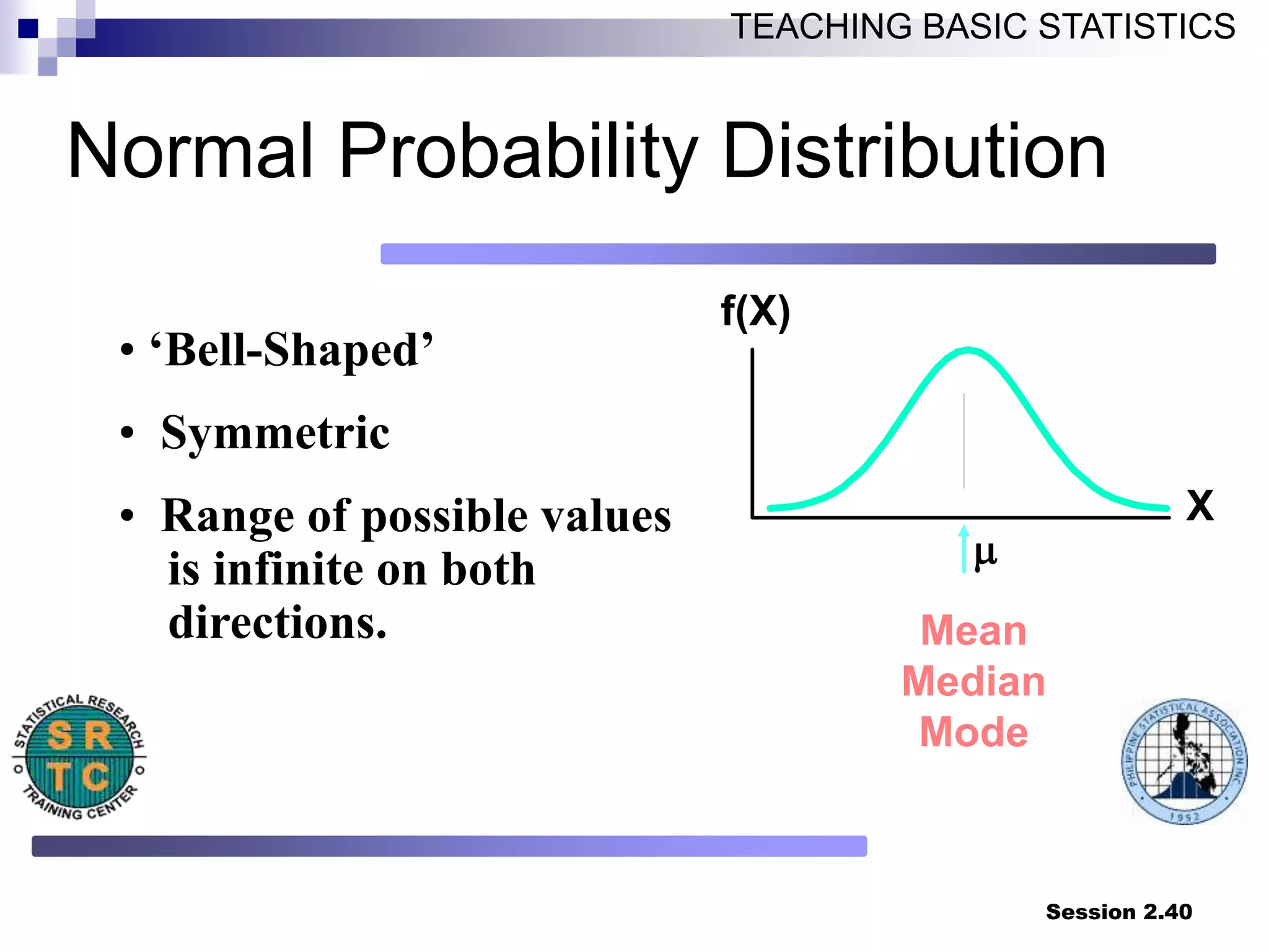
• ‘Bell-Shaped’
• Symmetric
• Range of possible values
is infinite on both
directions. Mean
Median
Mode
X
f(X)
m
Normal Probability Distribution
41.
Session 2.41
TEACHING BASICSTATISTICS
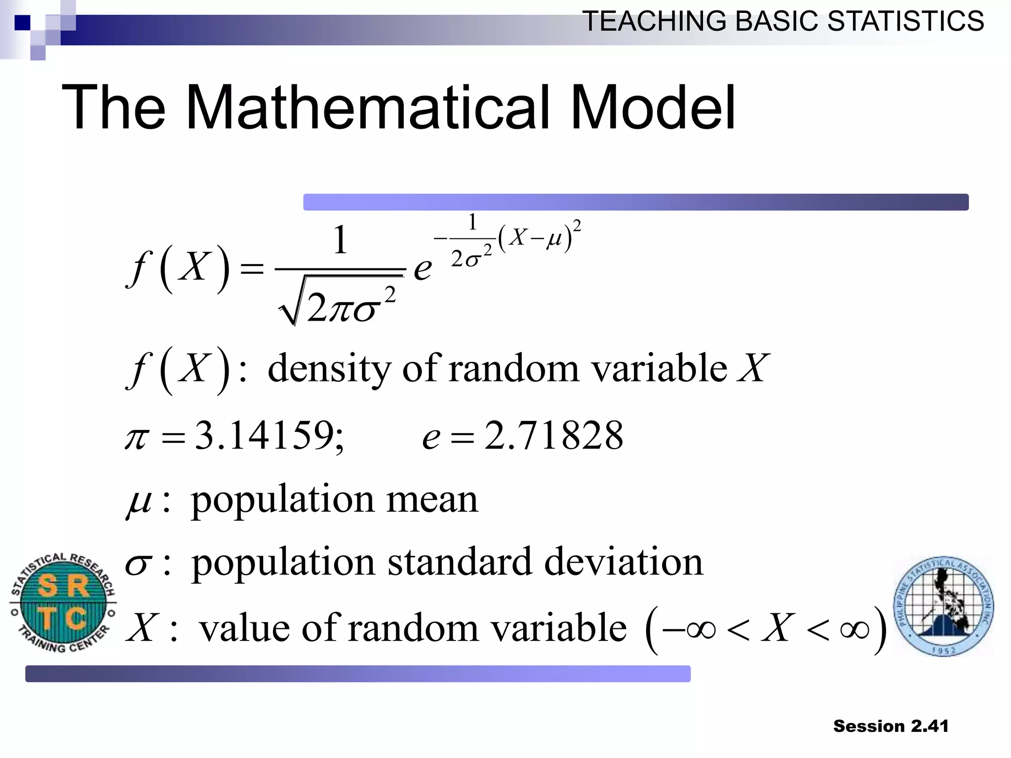
The Mathematical Model
2
1
2
2
1
2
: density of random variable
3.14159; 2.71828
: population mean
: population standard deviation
: value of random variable
X
f X e
f X X
e
X X
m
m
42.
Session 2.42
TEACHING BASICSTATISTICS
THE NORMAL CURVE
0.00
0.05
0.10
0.15
0.20
0.25
-15 -10 -5 0 5 10 15 20
Two normal distributions with the same mean but
different variances.
N(5,4)
N(5,9)
43.
Session 2.43
TEACHING BASICSTATISTICS
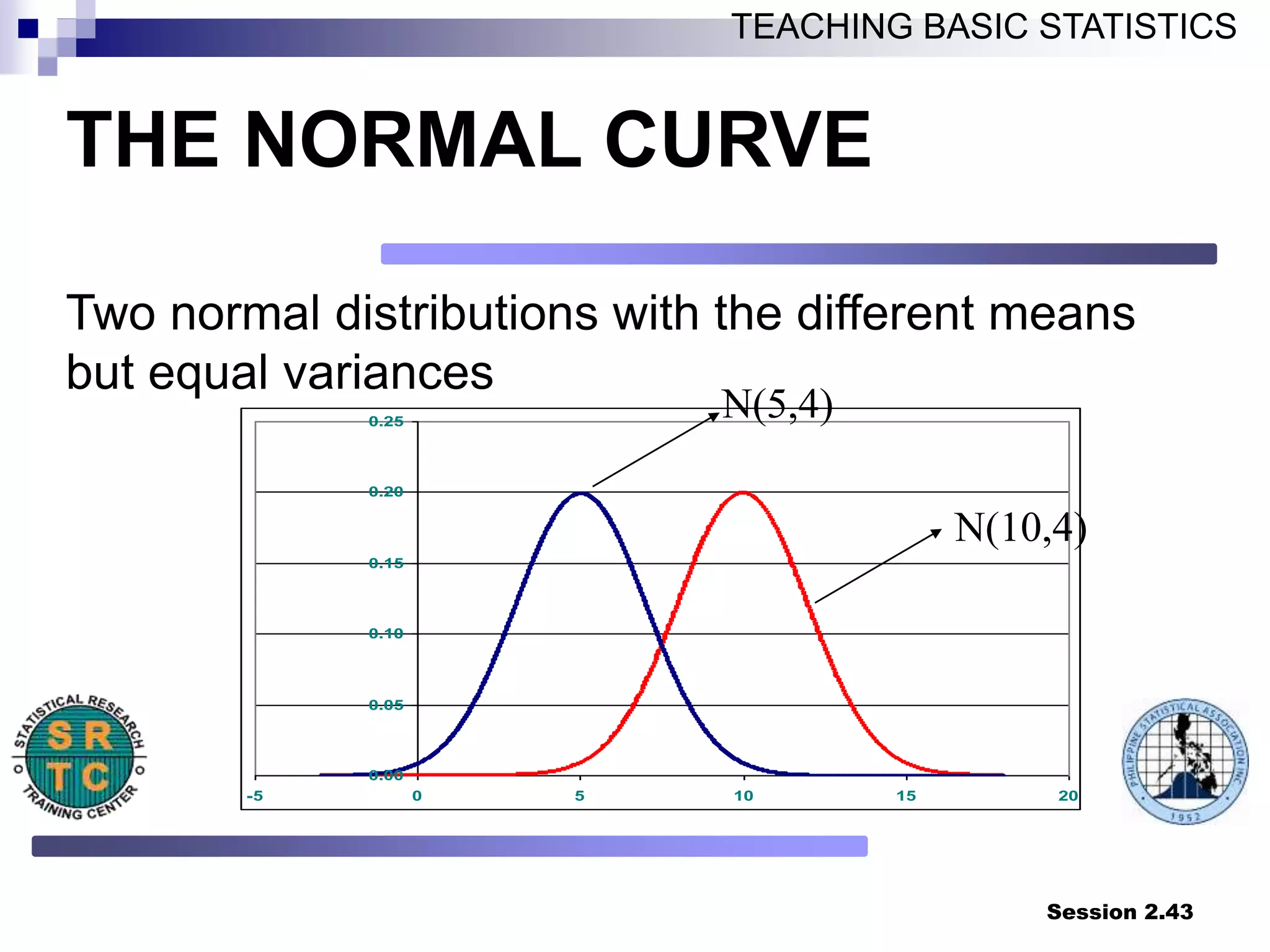
Two normal distributions with the different means
but equal variances
0.00
0.05
0.10
0.15
0.20
0.25
-5 0 5 10 15 20
N(5,4)
N(10,4)
THE NORMAL CURVE
44.
Session 2.44
TEACHING BASICSTATISTICS
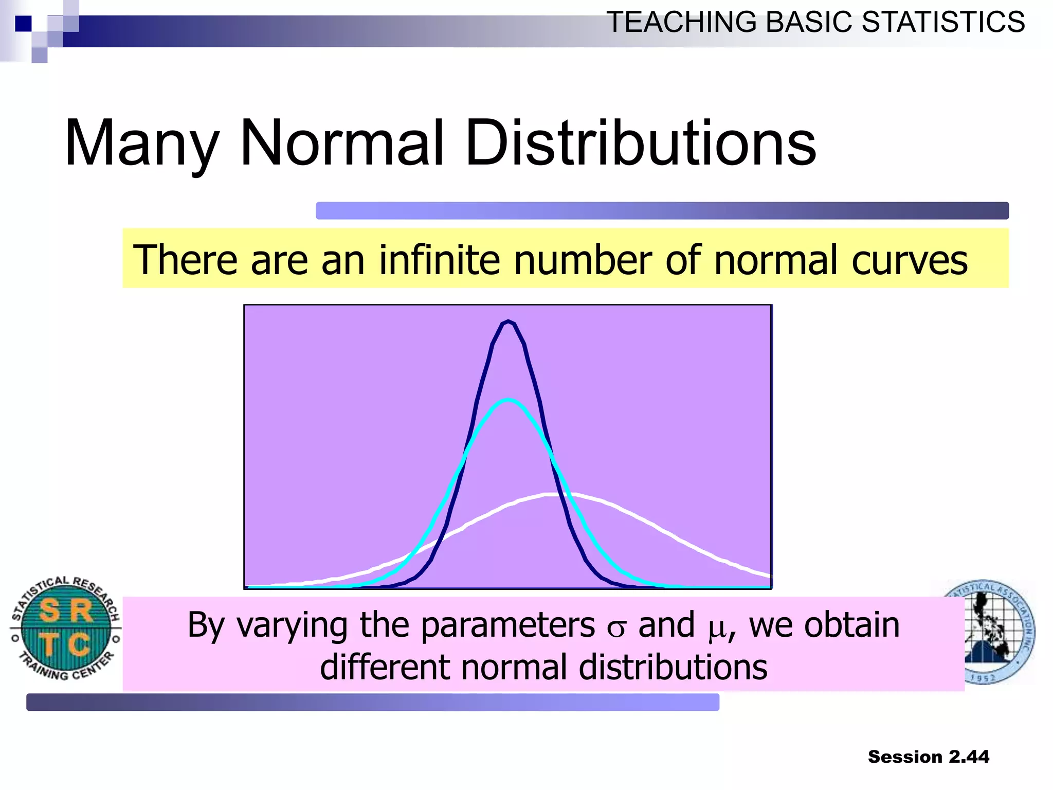
By varying the parameters and m, we obtain
different normal distributions
There are an infinite number of normal curves
Many Normal Distributions
45.
Session 2.45
TEACHING BASICSTATISTICS
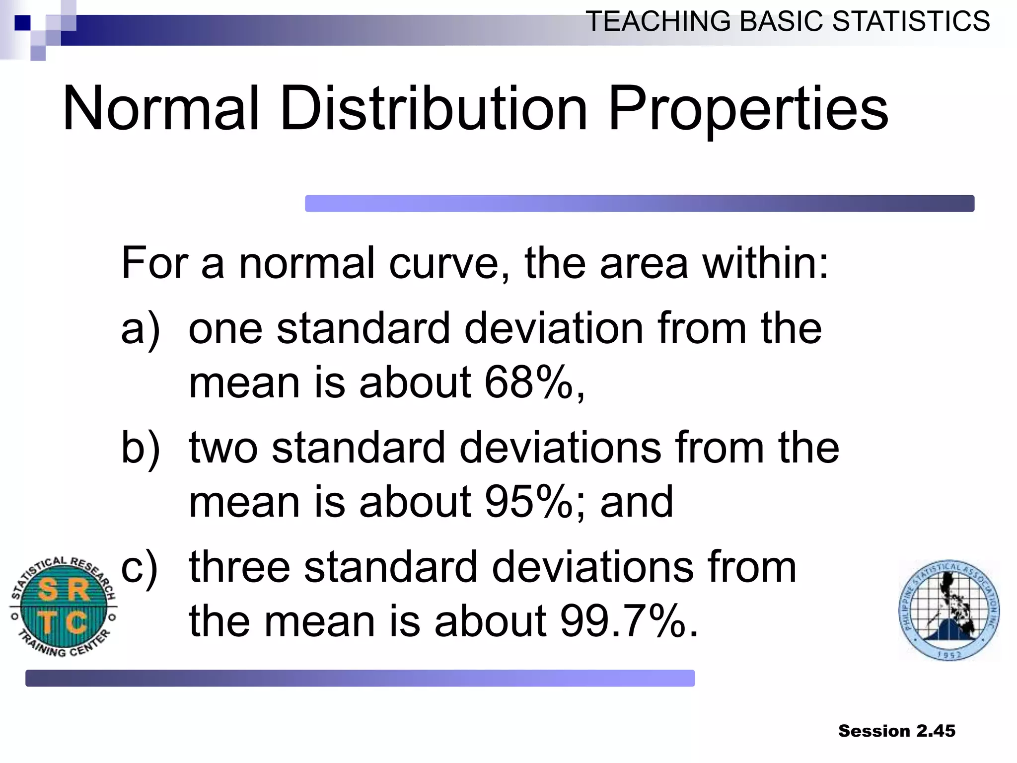
Normal Distribution Properties
For a normal curve, the area within:
a) one standard deviation from the
mean is about 68%,
b) two standard deviations from the
mean is about 95%; and
c) three standard deviations from
the mean is about 99.7%.
46.
Session 2.46
TEACHING BASICSTATISTICS
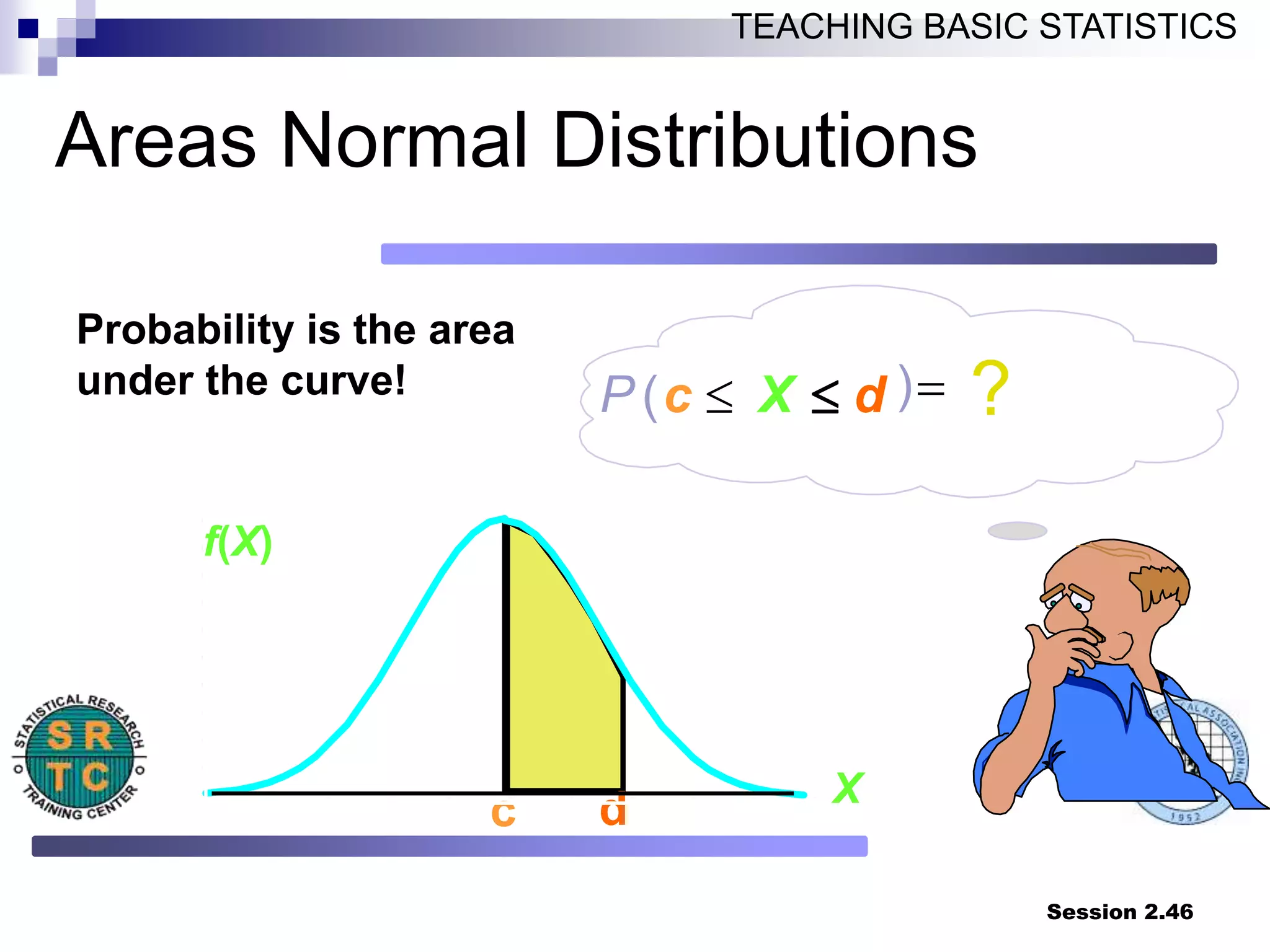
Probability is the area
under the curve!
c d X
f(X)
P c X d
( ) ?
Areas Normal Distributions
47.
Session 2.47
TEACHING BASICSTATISTICS
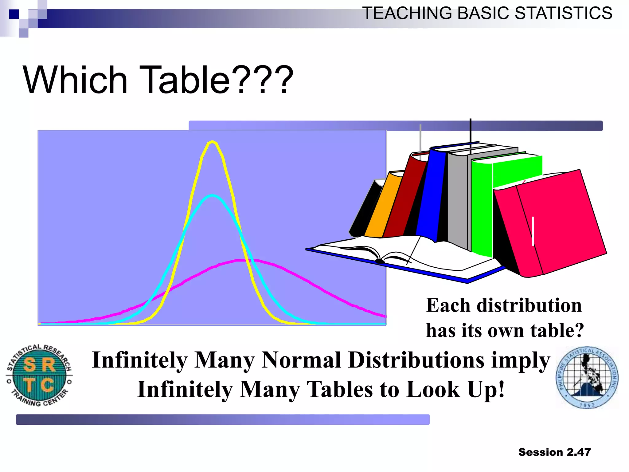
Infinitely Many Normal Distributions imply
Infinitely Many Tables to Look Up!
Each distribution
has its own table?
Which Table???
48.
Session 2.48
TEACHING BASICSTATISTICS
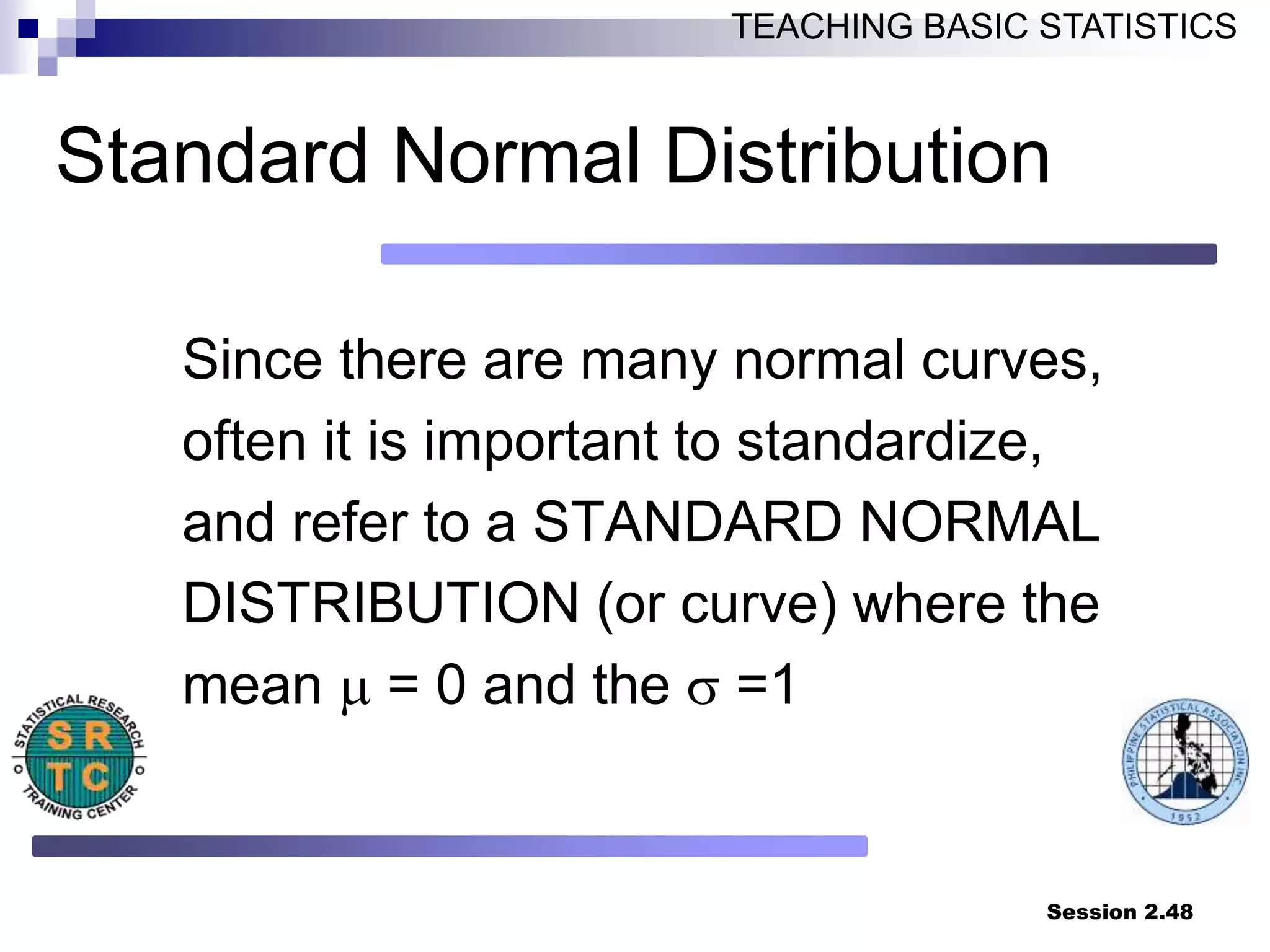
Standard Normal Distribution
Since there are many normal curves,
often it is important to standardize,
and refer to a STANDARD NORMAL
DISTRIBUTION (or curve) where the
mean m = 0 and the =1
49.
Session 2.49
TEACHING BASICSTATISTICS
THE Z-TABLE
P[Z z]
Examples:
1. P[Z 0] = 0.5
2. P[Z 1.25] = 0.8944
3. P[Z 1.96] = 0.9750
0 z
This table summarizes the cumulative probability
distribution for Z (i.e. P[Z z])
50.
Session 2.50
TEACHING BASICSTATISTICS
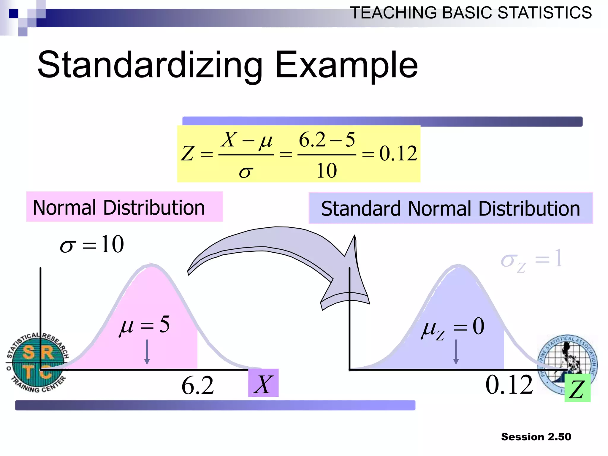
Standardizing Example
6.2 5
0.12
10
X
Z
m
Shaded Area Exaggerated
Normal Distribution
10
5
m
6.2 X
Standard Normal Distribution
Z
0
Z
m
0.12
1
Z
51.
Session 2.51
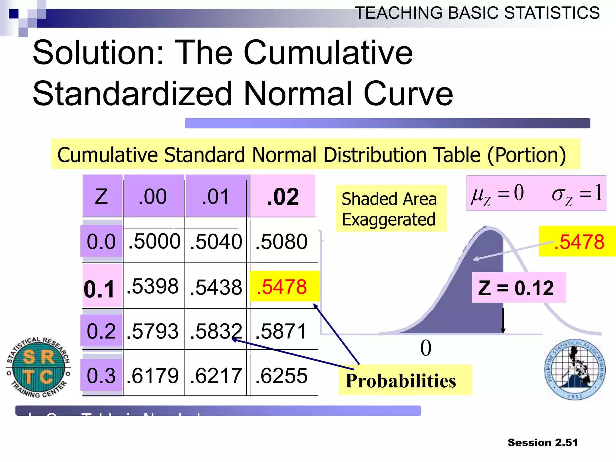
TEACHING BASICSTATISTICS
Solution: The Cumulative
Standardized Normal Curve
Z .00 .01
0.0 .5000 .5040 .5080
.5398 .5438
0.2 .5793 .5832 .5871
0.3 .6179 .6217 .6255
.5478
.02
0.1 .5478
Cumulative Standard Normal Distribution Table (Portion)
Probabilities
Shaded Area
Exaggerated
Only One Table is Needed
0 1
Z Z
m
Z = 0.12
0
52.
Session 2.52
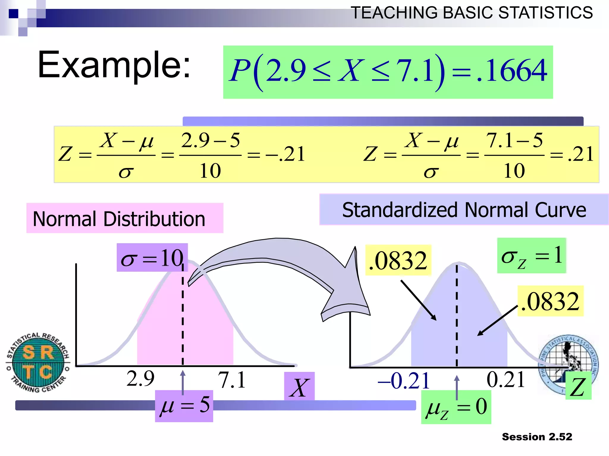
TEACHING BASICSTATISTICS
Normal Distribution Standardized Normal Curve
10
1
Z
5
m
7.1 X Z
0
Z
m
0.21
2.9 5 7.1 5
.21 .21
10 10
X X
Z Z
m m
2.9 0.21
.0832
2.9 7.1 .1664
P X
.0832
Shaded Area Exaggerated
Example:
53.
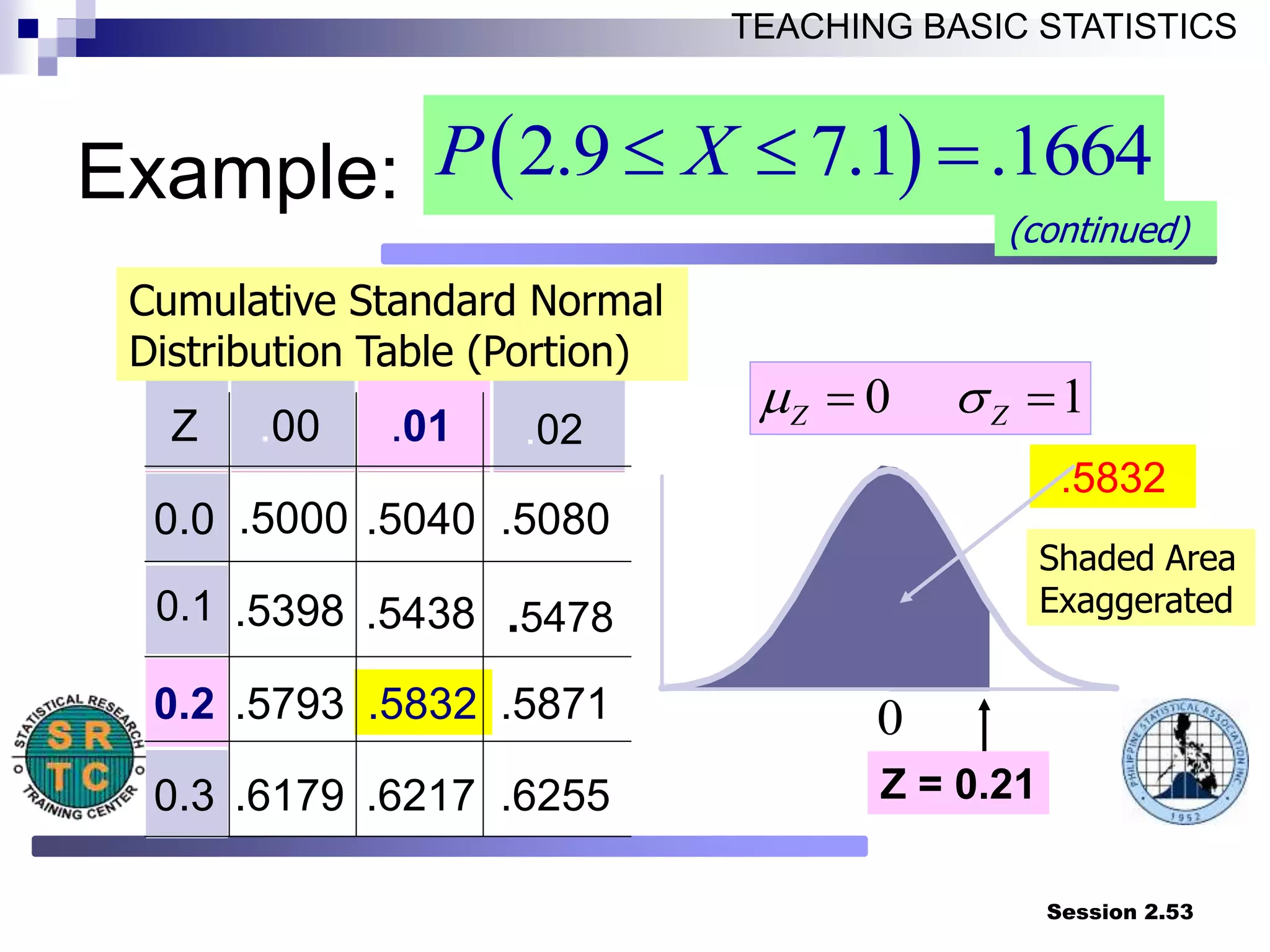
Session 2.53
TEACHING BASICSTATISTICS
Z .00 .01
0.0 .5000 .5040 .5080
.5398 .5438
0.2 .5793 .5832 .5871
0.3 .6179 .6217 .6255
.5832
.02
0.1 .5478
Cumulative Standard Normal
Distribution Table (Portion)
Shaded Area
Exaggerated
0 1
Z Z
m
Z = 0.21
(continued)
0
2.9 7.1 .1664
P X
Example:
54.
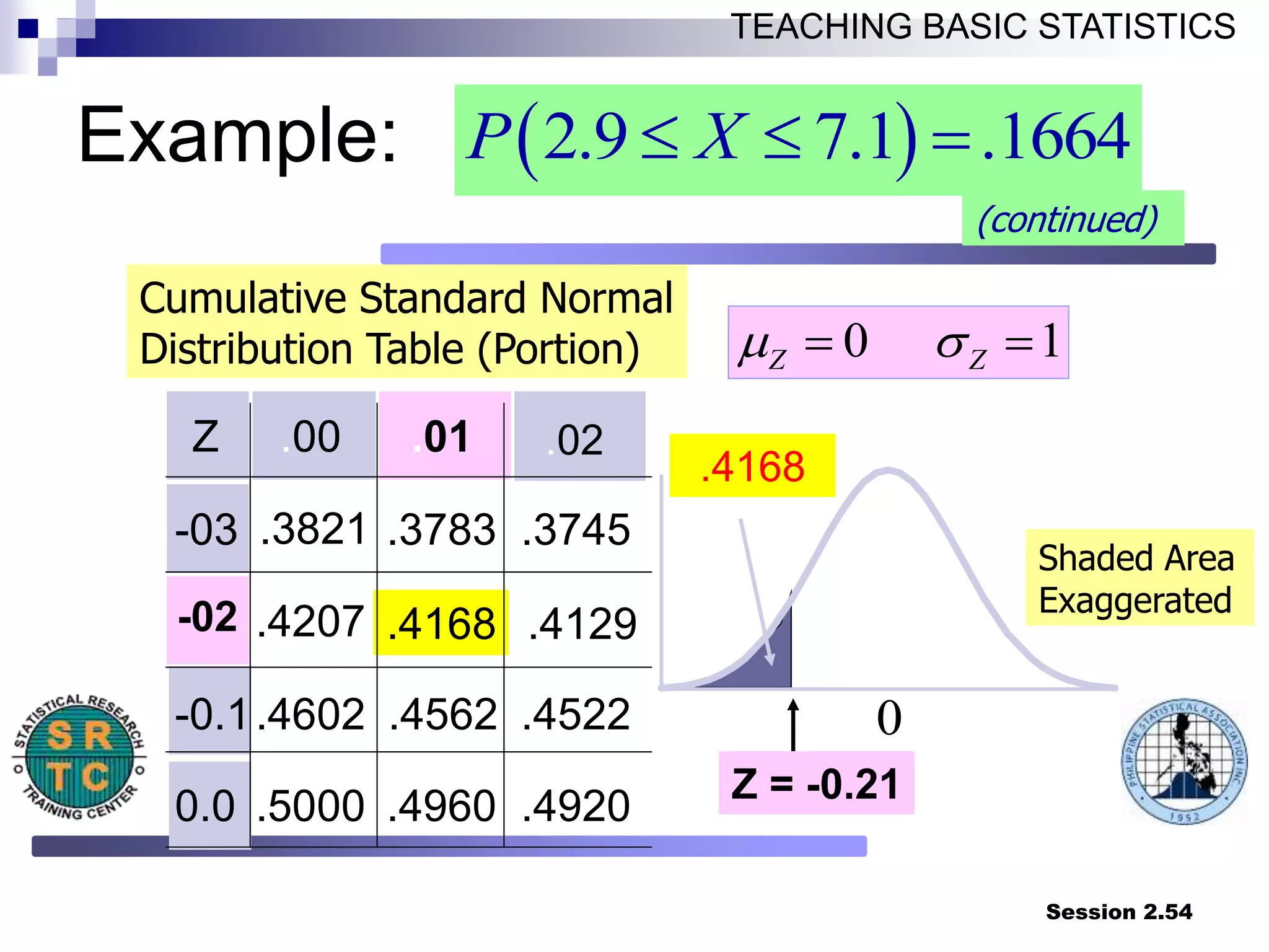
Session 2.54
TEACHING BASICSTATISTICS
Z .00 .01
-03 .3821 .3783 .3745
.4207 .4168
-0.1.4602 .4562 .4522
0.0 .5000 .4960 .4920
.4168
.02
-02 .4129
Cumulative Standard Normal
Distribution Table (Portion)
Shaded Area
Exaggerated
0 1
Z Z
m
Z = -0.21
2.9 7.1 .1664
P X
(continued)
0
Example:
55.
Session 2.55
TEACHING BASICSTATISTICS
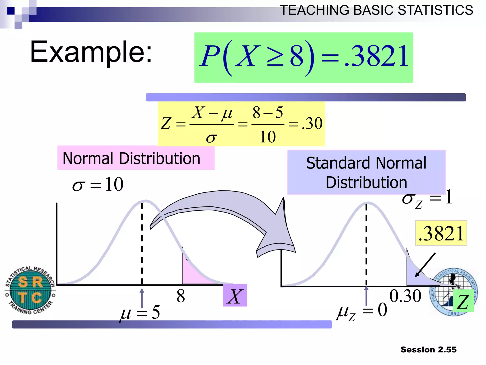
8 .3821
P X
Normal Distribution Standard Normal
Distribution
Shaded Area Exaggerated
10
1
Z
5
m
8 X Z
0
Z
m
0.30
8 5
.30
10
X
Z
m
.3821
Example:
56.
Session 2.56
TEACHING BASICSTATISTICS
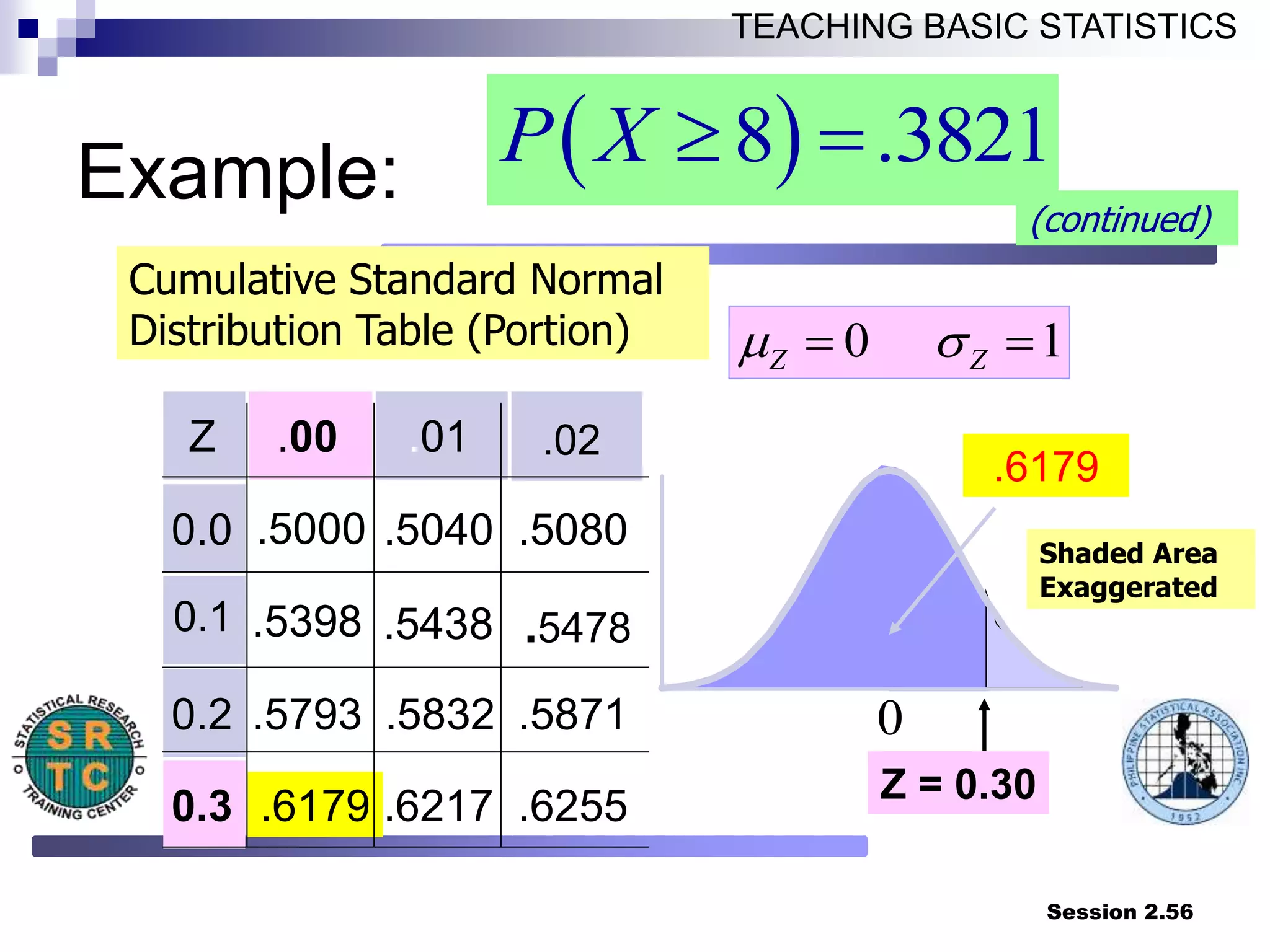
(continued)
Z .00 .01
0.0 .5000 .5040 .5080
.5398 .5438
0.2 .5793 .5832 .5871
0.3 .6179 .6217 .6255
.6179
.02
0.1 .5478
Cumulative Standard Normal
Distribution Table (Portion)
Shaded Area
Exaggerated
0 1
Z Z
m
Z = 0.30
0
8 .3821
P X
Example:
57.
Session 2.57
TEACHING BASICSTATISTICS
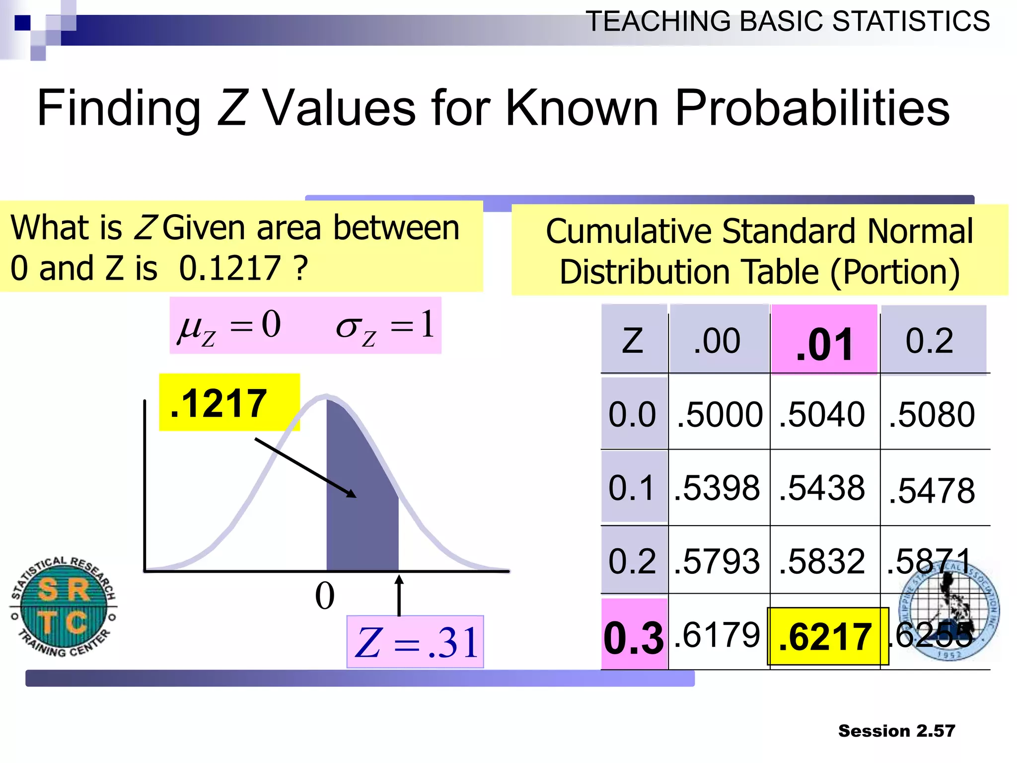
.1217
Finding Z Values for Known Probabilities
Z .00 0.2
0.0 .5000 .5040 .5080
0.1 .5398 .5438 .5478
0.2 .5793 .5832 .5871
.6179 .6255
.01
0.3
Cumulative Standard Normal
Distribution Table (Portion)
What is Z Given area between
0 and Z is 0.1217 ?
Shaded Area
Exaggerated
.6217
0 1
Z Z
m
.31
Z
0
58.
Session 2.58
TEACHING BASICSTATISTICS
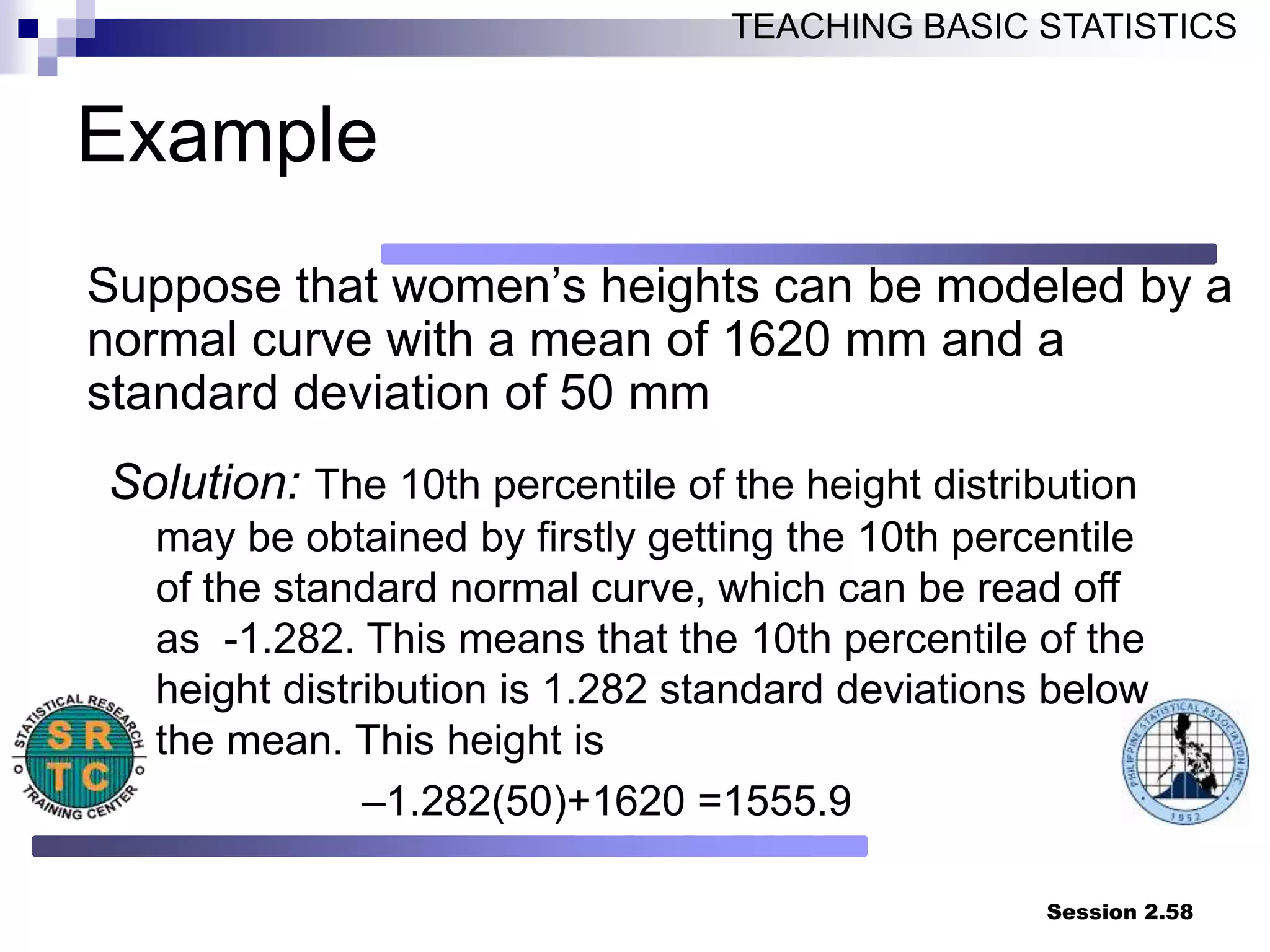
Example
Suppose that women’s heights can be modeled by a
normal curve with a mean of 1620 mm and a
standard deviation of 50 mm
Solution: The 10th percentile of the height distribution
may be obtained by firstly getting the 10th percentile
of the standard normal curve, which can be read off
as -1.282. This means that the 10th percentile of the
height distribution is 1.282 standard deviations below
the mean. This height is
–1.282(50)+1620 =1555.9
59.
Session 2.59
TEACHING BASICSTATISTICS
RULES IN COMPUTING PROBABILITIES
P[Z = a] = 0
P[Z a] can be obtained directly
from the Z-table
P[Z a] = 1 – P[Z a]
P[Z -a] = P[Z +a]
P[Z -a] = P[Z +a]
P[a1 Z a2] = P[Z a2] – P[Z a1]
![Session 2.2
TEACHING BASIC STATISTICS
Motivation for Studying Chance
Sample Statistic Estimates Population Parameter
e.g. Sample Mean X = 50 estimates Population Mean m
Questions:
1. How do we assess the reliability of our estimate?
2. What is an adequate sample size? [ We would expect a
large sample to give better estimates. Large samples
more costly.]](https://image.slidesharecdn.com/probabilityandprobabilitydistributions-220910103318-3c66fd6e/75/PROBABILITY-AND-PROBABILITY-DISTRIBUTIONS-ppt-2-2048.jpg)

![Session 2.24
TEACHING BASIC STATISTICS
UNEQUALLY LIKELY OUTCOME
ASSUMPTION
The outcomes have different
likelihood to occur.
The probability of an event E is
then computed as the sum of the
probabilities of the outcomes
found in the event E, that is,
P[E] = sum of p{e}
where e is an element of event E.](https://image.slidesharecdn.com/probabilityandprobabilitydistributions-220910103318-3c66fd6e/75/PROBABILITY-AND-PROBABILITY-DISTRIBUTIONS-ppt-24-2048.jpg)
![Session 2.25
TEACHING BASIC STATISTICS
ILLUSTRATION
S = {1, 2, 3, 4, 5, 6}
Assuming that the probability of each of the
outcomes 1,2, and 3 is 1/12 while each of the
outcomes 4, 5 and 6 has likelihood to occur
equal to 1/4.
The probability of an event of observing odd-
number of dots in a roll of a die is P[E1] = sum
of p{1}, p{3} and p{5} = 1/12 + 1/12 + 1/4 =
5/12.](https://image.slidesharecdn.com/probabilityandprobabilitydistributions-220910103318-3c66fd6e/75/PROBABILITY-AND-PROBABILITY-DISTRIBUTIONS-ppt-25-2048.jpg)
![Session 2.27
TEACHING BASIC STATISTICS
ILLUSTRATION
Suppose the experiment was done
for 100 times and it was observed
that an odd-number of dots occurred
60 times and even-number of dots
occurred 40 times.
The probability of an event of
observing odd-number of dots in a
roll of a die is the relative frequency
of the event or P[E1] = 60/100 = 0.6](https://image.slidesharecdn.com/probabilityandprobabilitydistributions-220910103318-3c66fd6e/75/PROBABILITY-AND-PROBABILITY-DISTRIBUTIONS-ppt-27-2048.jpg)
![Session 2.34
TEACHING BASIC STATISTICS
ILLUSTRATION
The probability distribution of the random variable, X defined
as the total number of dots on the upturned faces in a roll of
two dice, is presented as a table below:
X 2 3 4 5 6 7 8 9 10 11 12
P[X=x] 1/36 2/36 3/36 4/36 5/36 6/36 5/36 4/36 3/36 2/36 1/36
0.00
0.05
0.10
0.15
0.20
2 3 4 5 6 7 8 9 10 11 12
X = Total Number of Dots on the Upturned faces](https://image.slidesharecdn.com/probabilityandprobabilitydistributions-220910103318-3c66fd6e/75/PROBABILITY-AND-PROBABILITY-DISTRIBUTIONS-ppt-34-2048.jpg)


![Session 2.49
TEACHING BASIC STATISTICS
THE Z-TABLE
P[Z z]
Examples:
1. P[Z 0] = 0.5
2. P[Z 1.25] = 0.8944
3. P[Z 1.96] = 0.9750
0 z
This table summarizes the cumulative probability
distribution for Z (i.e. P[Z z])](https://image.slidesharecdn.com/probabilityandprobabilitydistributions-220910103318-3c66fd6e/75/PROBABILITY-AND-PROBABILITY-DISTRIBUTIONS-ppt-49-2048.jpg)
![Session 2.59
TEACHING BASIC STATISTICS
RULES IN COMPUTING PROBABILITIES
P[Z = a] = 0
P[Z a] can be obtained directly
from the Z-table
P[Z a] = 1 – P[Z a]
P[Z -a] = P[Z +a]
P[Z -a] = P[Z +a]
P[a1 Z a2] = P[Z a2] – P[Z a1]](https://image.slidesharecdn.com/probabilityandprobabilitydistributions-220910103318-3c66fd6e/75/PROBABILITY-AND-PROBABILITY-DISTRIBUTIONS-ppt-59-2048.jpg)


![[DSC Europe 25] Sara Polak - The Ancient Operating System: What Archaeology T...](https://cdn.slidesharecdn.com/ss_thumbnails/3vch2p6tttdnwhsgazoz-3-sara-polak-smart-cities-251208152532-64404202-thumbnail.jpg?width=640&height=640&fit=bounds)
![[DSC Europe 25] Imai Jen-La Plante - The New Generation: AI and the Future of...](https://cdn.slidesharecdn.com/ss_thumbnails/kxi8t2l5rggivgcenyba-1-jenlaplante-dsc-251208152532-d1e076c2-thumbnail.jpg?width=640&height=640&fit=bounds)
![[DSC Europe 25] Dobrica Cosic - Savings by the Second: How Dynamic Pricing an...](https://cdn.slidesharecdn.com/ss_thumbnails/znp09f3smtqz3w2sq6wn-1-dobrica-cosic-savings-by-the-second-how-dynamic-pricing-and-smart-data-are-bu-251208151905-26e6f41e-thumbnail.jpg?width=640&height=640&fit=bounds)


![[DSC Europe 25] Katherine Forrest - AI NOW: Understanding the Velocity of Cha...](https://cdn.slidesharecdn.com/ss_thumbnails/wvvbruqfrci0sfq9xwgb-4-251212104007-e5ad1987-thumbnail.jpg?width=640&height=640&fit=bounds)
![[DSC Europe 25] Dusan Jovicic - AI Story: From on-prem to cloud and back agai...](https://cdn.slidesharecdn.com/ss_thumbnails/8kp49m6uq22ifnbwhfnk-2-251205085715-964d11a6-thumbnail.jpg?width=640&height=640&fit=bounds)

![[DSC Europe 25] Jovan Bogicevic - Legacy to AI-Driven Defense: Transforming D...](https://cdn.slidesharecdn.com/ss_thumbnails/rsarluadt563hntyfc8q-3-251211083849-3e7bc4c0-thumbnail.jpg?width=640&height=640&fit=bounds)
![[DSC Europe 25] Dragan Vucic - Building the Learning Organization - How AI Tr...](https://cdn.slidesharecdn.com/ss_thumbnails/8brigo2sbu6qur6gxrra-7-251205085715-6ae07d24-thumbnail.jpg?width=640&height=640&fit=bounds)

![[DSC Europe 25] Goran Obradovic - The Rise of Sovereign AI: Building the Regi...](https://cdn.slidesharecdn.com/ss_thumbnails/7nw2xxixrxqdxvrb5wca-6-251205085714-ab09a2ac-thumbnail.jpg?width=640&height=640&fit=bounds)
![[DSC Europe 25] Branko Dzakula - From Defense to Attack: How AI Redefines Cyb...](https://cdn.slidesharecdn.com/ss_thumbnails/80bdzdxpr3ky2g0qvyk9-8-251211083048-ce5fc1ee-thumbnail.jpg?width=640&height=640&fit=bounds)
![[DSC Europe 25] Vladimir Jelic - The AI-Driven Security Shift From Reactive D...](https://cdn.slidesharecdn.com/ss_thumbnails/6g5gj25mtjwayniqem1t-6-251209104645-7a5a5fc6-thumbnail.jpg?width=640&height=640&fit=bounds)
![[DSC Europe 25] Dusan Pavlov - There Is No Spoon: Inferring Vision from Neura...](https://cdn.slidesharecdn.com/ss_thumbnails/wg0v1umoqjm4nnbd3p0v-there-is-no-spoon-251205085715-6d81d6c5-thumbnail.jpg?width=640&height=640&fit=bounds)

![[DSC Europe 25] Milan Zdravkovic - The road less traveled in District Heating...](https://cdn.slidesharecdn.com/ss_thumbnails/nfaboniqwsz4ucyctnmy-2-milan-zdravkovic-dsc2025-the-road-less-traveled-in-district-heating-operation-251208151905-f56388a5-thumbnail.jpg?width=640&height=640&fit=bounds)

![[DSC Europe 25] Bassam Maharmeh - Artificial Intelligence: Opportunities and ...](https://cdn.slidesharecdn.com/ss_thumbnails/thhfmr2fqpawzj7hsjpg-5-251211083048-2c23204f-thumbnail.jpg?width=640&height=640&fit=bounds)
