Chap03 probability

Chapter 3
Probability
Statistics for
Business and Economics
7th Edition
Copyright © 2010 Pearson Education, Inc. Publishing as Prentice Hall Ch. 3-1

Chapter Goals
After completing this chapter, you should be
able to:
 Explain basic probability concepts and definitions
 Use a Venn diagram or tree diagram to illustrate
simple probabilities
 Apply common rules of probability
 Compute conditional probabilities
 Determine whether events are statistically
independent
 Use Bayes’ Theorem for conditional probabilities

Important Terms
 Random Experiment – a process leading to an
uncertain outcome
 Basic Outcome – a possible outcome of a
random experiment
 Sample Space – the collection of all possible
outcomes of a random experiment
 Event – any subset of basic outcomes from the
sample space
3.1

Important Terms
 Intersection of Events – If A and B are two
events in a sample space S, then the
intersection, A ∩ B, is the set of all outcomes in
S that belong to both A and B
(continued)
A BAB
S

Important Terms
 A and B are Mutually Exclusive Events if they
have no basic outcomes in common
 i.e., the set A ∩ B is empty
(continued)
A B
S

Important Terms
 Union of Events – If A and B are two events in a
sample space S, then the union, A U B, is the
set of all outcomes in S that belong to either
A or B
(continued)
A B
The entire shaded
area represents
A U B
S

Important Terms
 Events E1, E2, … Ek are Collectively Exhaustive
events if E1 U E2 U . . . U Ek = S
 i.e., the events completely cover the sample space
 The Complement of an event A is the set of all
basic outcomes in the sample space that do not
belong to A. The complement is denoted
(continued)
A
A
S
A

Examples
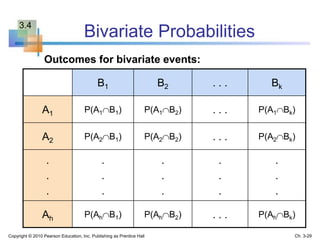
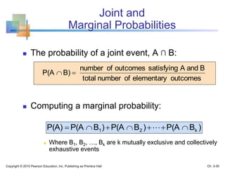
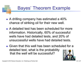
Let the Sample Space be the collection of
all possible outcomes of rolling one die:
S = [1, 2, 3, 4, 5, 6]
Let A be the event “Number rolled is even”
Let B be the event “Number rolled is at least 4”
Then
A = [2, 4, 6] and B = [4, 5, 6]

Examples
(continued)
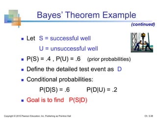
S = [1, 2, 3, 4, 5, 6] A = [2, 4, 6] B = [4, 5, 6]
5]3,[1,A 
6][4,BA 
6]5,4,[2,BA 
S6]5,4,3,2,[1,AA 
Complements:
Intersections:
Unions:
[5]BA 
3]2,[1,B 

Examples
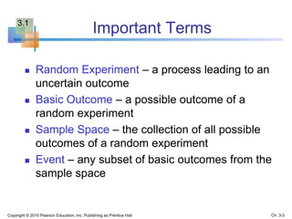
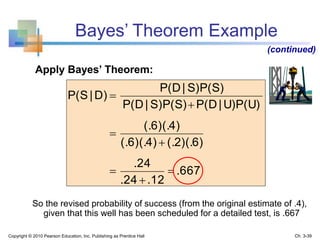
 Mutually exclusive:
 A and B are not mutually exclusive
 The outcomes 4 and 6 are common to both
 Collectively exhaustive:
 A and B are not collectively exhaustive
 A U B does not contain 1 or 3
(continued)
S = [1, 2, 3, 4, 5, 6] A = [2, 4, 6] B = [4, 5, 6]

Probability
 Probability – the chance that
an uncertain event will occur
(always between 0 and 1)
0 ≤ P(A) ≤ 1 For any event A
Certain
Impossible
.5
1
0
3.2

Assessing Probability
 There are three approaches to assessing the
probability of an uncertain event:
1. classical probability
 Assumes all outcomes in the sample space are equally likely to
occur
spacesampletheinoutcomesofnumbertotal
eventthesatisfythatoutcomesofnumber
N
N
Aeventofyprobabilit A


Counting the Possible Outcomes
 Use the Combinations formula to determine the
number of combinations of n things taken k at a
time
 where
 n! = n(n-1)(n-2)…(1)
 0! = 1 by definition
k)!(nk!
n!
Cn
k



Assessing Probability
Three approaches (continued)
2. relative frequency probability
 the limit of the proportion of times that an event A occurs in a large
number of trials, n
3. subjective probability
an individual opinion or belief about the probability of occurrence
populationtheineventsofnumbertotal
Aeventsatisfythatpopulationtheineventsofnumber
n
n
Aeventofyprobabilit A


Probability Postulates
1. If A is any event in the sample space S, then
2. Let A be an event in S, and let Oi denote the basic
outcomes. Then
(the notation means that the summation is over all the basic outcomes in A)
3. P(S) = 1
1P(A)0 
)P(OP(A)
A
i

Probability Rules
 The Complement rule:
 The Addition rule:
 The probability of the union of two events is
1)AP(P(A)i.e., P(A)1)AP( 
B)P(AP(B)P(A)B)P(A 
3.3

A Probability Table
B
A
A
B
)BP(A 
)BAP( B)AP( 
P(A)B)P(A
)AP(
)BP(P(B) 1.0P(S) 
Probabilities and joint probabilities for two
events A and B are summarized in this table:

Addition Rule Example
Consider a standard deck of 52 cards, with four
suits: ♥ ♣ ♦ ♠
Let event A = card is an Ace
Let event B = card is from a red suit

Addition Rule Example
P(Red U Ace) = P(Red) + P(Ace) - P(Red ∩ Ace)
= 26/52 + 4/52 - 2/52 = 28/52
Don’t count
the two red
aces twice!
Black
Color
Type Red Total
Ace 2 2 4
Non-Ace 24 24 48
Total 26 26 52
(continued)

Conditional Probability
 A conditional probability is the probability of one
event, given that another event has occurred:
P(B)
B)P(A
B)|P(A


P(A)
B)P(A
A)|P(B


The conditional
probability of A
given that B has
occurred
The conditional
probability of B
given that A has
occurred

Conditional Probability Example
 What is the probability that a car has a CD
player, given that it has AC ?
i.e., we want to find P(CD | AC)
 Of the cars on a used car lot, 70% have air
conditioning (AC) and 40% have a CD player
(CD). 20% of the cars have both.

No CDCD Total
AC .2 .5 .7
No AC .2 .1 .3
Total .4 .6 1.0
conditioning (AC) and 40% have a CD player (CD).
20% of the cars have both.
.2857
.7
.2
P(AC)
AC)P(CD
AC)|P(CD 


(continued)

No CDCD Total
AC .2 .5 .7
No AC .2 .1 .3
Total .4 .6 1.0
 Given AC, we only consider the top row (70% of the cars). Of
these, 20% have a CD player. 20% of 70% is 28.57%.
.2857
.7
.2
P(AC)
AC)P(CD
AC)|P(CD 


(continued)

Multiplication Rule
 Multiplication rule for two events A and B:
 also
P(B)B)|P(AB)P(A 
P(A)A)|P(BB)P(A 

Multiplication Rule Example
P(Red ∩ Ace) = P(Red| Ace)P(Ace)
Black
Color
Type Red Total
Ace 2 2 4
Non-Ace 24 24 48
Total 26 26 52
52
2
52
4
4
2













52
2
cardsofnumbertotal
aceandredarethatcardsofnumber


Statistical Independence
 Two events are statistically independent
if and only if:
 Events A and B are independent when the probability of one
event is not affected by the other event
 If A and B are independent, then
P(A)B)|P(A 
P(B)P(A)B)P(A 
P(B)A)|P(B 
if P(B)>0
if P(A)>0

Statistical Independence Example
No CDCD Total
AC .2 .5 .7
No AC .2 .1 .3
Total .4 .6 1.0
conditioning (AC) and 40% have a CD player (CD).
20% of the cars have both.
 Are the events AC and CD statistically independent?

Statistical Independence Example
No CDCD Total
AC .2 .5 .7
No AC .2 .1 .3
Total .4 .6 1.0
(continued)
P(AC ∩ CD) = 0.2
P(AC) = 0.7
P(CD) = 0.4
P(AC)P(CD) = (0.7)(0.4) = 0.28
P(AC ∩ CD) = 0.2 ≠ P(AC)P(CD) = 0.28
So the two events are not statistically independent

Bivariate Probabilities
B1 B2 . . . Bk
A1 P(A1B1) P(A1B2) . . . P(A1Bk)
A2 P(A2B1) P(A2B2) . . . P(A2Bk)
.
.
.
.
.
.
.
.
.
.
.
.
.
.
.
Ah P(AhB1) P(AhB2) . . . P(AhBk)
Outcomes for bivariate events:
3.4

Joint and
Marginal Probabilities
 The probability of a joint event, A ∩ B:
 Computing a marginal probability:
 Where B1, B2, …, Bk are k mutually exclusive and collectively
exhaustive events
outcomeselementaryofnumbertotal
BandAsatisfyingoutcomesofnumber
B)P(A 
)BP(A)BP(A)BP(AP(A) k21  

Marginal Probability Example
P(Ace)
Black
Color
Type Red Total
Ace 2 2 4
Non-Ace 24 24 48
Total 26 26 52
52
4
52
2
52
2
Black)P(AceRed)P(Ace 

Using a Tree Diagram
P(AC ∩ CD) = .2
P(AC ∩ CD) = .5
P(AC ∩ CD) = .1
P(AC ∩ CD) = .2
7.
5.
3.
2.
3.
1.
All
Cars
7.
2.
Given AC or
no AC:

Odds
 The odds in favor of a particular event are
given by the ratio of the probability of the
event divided by the probability of its
complement
 The odds in favor of A are
)AP(
P(A)
P(A)1-
P(A)
odds 

Odds: Example
 Calculate the probability of winning if the odds
of winning are 3 to 1:
 Now multiply both sides by 1 – P(A) and solve for P(A):
3 x (1- P(A)) = P(A)
3 – 3P(A) = P(A)
3 = 4P(A)
P(A) = 0.75
P(A)1-
P(A)
1
3
odds 

Overinvolvement Ratio
 The probability of event A1 conditional on event B1
divided by the probability of A1 conditional on activity B2
is defined as the overinvolvement ratio:
 An overinvolvement ratio greater than 1 implies that
event A1 increases the conditional odds ration in favor
of B1:
)B|P(A
)B|P(A
21
11
)P(B
)P(B
)A|P(B
)A|P(B
2
1
12
11


Bayes’ Theorem Example
 A drilling company has estimated a 40%
chance of striking oil for their new well.
 A detailed test has been scheduled for more
information. Historically, 60% of successful
wells have had detailed tests, and 20% of
unsuccessful wells have had detailed tests.
 Given that this well has been scheduled for a
detailed test, what is the probability
that the well will be successful?

 Let S = successful well
U = unsuccessful well
 P(S) = .4 , P(U) = .6 (prior probabilities)
 Define the detailed test event as D
 Conditional probabilities:
P(D|S) = .6 P(D|U) = .2
 Goal is to find P(S|D)
(continued)

So the revised probability of success (from the original estimate of .4),
given that this well has been scheduled for a detailed test, is .667
667.
12.24.
24.
)6)(.2(.)4)(.6(.
)4)(.6(.
U)P(U)|P(DS)P(S)|P(D
S)P(S)|P(D
D)|P(S







(continued)
Apply Bayes’ Theorem:

Chapter Summary
 Defined basic probability concepts
 Sample spaces and events, intersection and union
of events, mutually exclusive and collectively
exhaustive events, complements
 Examined basic probability rules
 Complement rule, addition rule, multiplication rule
 Defined conditional, joint, and marginal probabilities
 Reviewed odds and the overinvolvement ratio
 Defined statistical independence
 Discussed Bayes’ theorem

Chap03 probability

More Related Content

What's hot

Similar to Chap03 probability

More from Judianto Nugroho

Recently uploaded

Chap03 probability