This document contains solutions to problems from Chapter 9. It provides worked examples of calculating voltages and currents in circuits containing operational amplifiers. Key steps and results are shown for multiple circuit configurations, including calculating voltage gains, identifying resistor values, and determining output voltages and currents given input signals. Operational amplifier circuits with one, two and multiple stages are analyzed using relevant equations.

1. Chapter 9
Problem Solutions
9.1
(a)
vO = Ad ( v2 − v1 )
( )
1 = Ad 10−3 − ( −10−3 ) ⇒ Ad = 500
(b)
1 = 500 ( v2 − 10−3 ) = 1 + 0.5 = 500v2
v2 = 3 mV
(c)
5 = 500 (1 − v1 ) ⇒ 500v1 = 495
v1 = 0.990 V
(d) vO = 0
(e)
− 3 = 500 ( v2 − ( −0.5 ) )
−250 − 3 = 500v2
v2 = −0.506 V
9.2
(a)
⎛ ⎞
⎟ vI = ( 0.49975 × 10 ) ( 3)
1 −3
v2 = ⎜
⎝ 1 + 2000 ⎠
v2 = 1.49925 × 10−3
vO = Aod ( v2 − v1 ) = ( 5 × 103 )(1.49925 × 10−3 − 0 )
vO = 7.49625 V
(b)
vO = Aod ( v2 − v1 )
3 = Aod (1.49925 × 10−3 − 0 )
Aod = 2 × 103
9.3
R2
Av = − = −12 ⇒ R2 = 12 R1
R1
Ri = R1 = 25 kΩ ⇒ R2 = (12 )( 25 ) = 300 kΩ
9.3
(a) v2 = 3.00 V
(b)
vO = Aod ( v2 − v1 )
2.500 = Aod ( 3.010 − 3.00 )
Aod = 250
9.4

2. ⎛ Ri ⎞
vid = ⎜ ⎟ vI
⎝ Ri + 25 ⎠
⎛ Ri ⎞
0.790 = ⎜ ⎟ ( 0.80 )
⎝ Ri + 25 ⎠
0.9875 ( Ri + 25 ) = Ri
24.6875 = 0.0125 Ri
Ri = 1975 K
9.5
200 ⎫
Av = − = −10 ⎪
20
⎪
and ⎬ for each case
Ri = 20 kΩ ⎪
⎪
⎭
9.6
a.
100
Av = − = −10
10
Ri = R1 = 10 kΩ
b.
100 100
Av = − = −5
10
Ri = R1 = 10 kΩ
c.
100
Av = − = −5
10 + 10
Ri = 10 + 10 = 20 K
9.7

3. vI 0.5
I1 = ⇒ R1 = ⇒ R1 = 5 K
R1 0.1
R2
= 15 ⇒ R2 = 75 K
R1
9.8
R2
Av = −
R1
(a) Av = −10
(b) Av = −1
(c) Av = −0.20
(d) Av = −10
(e) Av = −2
(f) Av = −1
9.9
R2
Av = −
R1
(a) R1 = 20 K, R2 = 40 K
(b) R1 = 20 K, R2 = 200 K
(c) R1 = 20 K, R2 = 1000 K
(d) R1 = 80 K, R2 = 20 K
9.10
R2
Av = − = −8 ⇒ R2 = 8 R1
R1
1
For vI = −1, i1 = = 15 μ A ⇒ R1 = 66.7 kΩ ⇒ R2 = 533.3 kΩ
R1
9.11
R2
Av = − = −30 ⇒ R2 = 30 R1
R1
Set R2 = 1 MΩ ⇒ R1 = 33.3 kΩ
9.12
a.
R2 1.05R2 ⎛R ⎞
Av = ⇒ = 1.105 ⎜ 2 ⎟
R1 0.95 R1 ⎝ R1 ⎠
0.95R2 ⎛R ⎞
= 0.905 ⎜ 2 ⎟
1.05R1 ⎝ R1 ⎠
Deviation in gain is +10.5% and − 9.5%
b.
1.01R2 ⎛R ⎞ 0.99 R2 ⎛R ⎞
Av ⇒ = 1.02 ⎜ 2 ⎟ ⇒ = 0.98 ⎜ 2 ⎟
0.99 R1 ⎝ R1 ⎠ 1.01R1 ⎝ R1 ⎠
Deviation in gain = ±2%
9.13
(a)

4. vO −15
Av = = = −15
vl 1
vO = −15vl ⇒ vO = −150sin ω t ( mV )
(b)
vI
i2 = i1 = = 10sin ω t ( μ A )
R1
vO
iL = ⇒ iL = −37.5sin ω t ( μ A )
RL
iO = iL − i2
iO = −47.5sin ω t ( μ A )
9.14
R2
Av = −
R1 + R5
Av = −30 ± 2.5% ⇒ 29.25 ≤ Av ≤ 30.75
R2 R2
So = 29.25 and = 30.75
R1 + 2 R1 + 1
We have 29.25 ( R1 + 2 ) = 30.75 ( R1 + 1)
Which yields R1 = 18.5 k Ω and R2 = 599.6 k Ω
For vI = 25 mV , then 0.731 ≤ vO ≤ 0.769 V
9.15
R2 120
vO1 = − , vI = − ( 0.2 ) ⇒ vO1 = −1.2 V
R1 20
R4 ⎛ −75 ⎞
vO = − , vO1 = ⎜ ⎟ ( −1.2 ) ⇒ vO = +6 V
R3 ⎝ 15 ⎠
0.2
i1 = i2 = ⇒ i1 = i2 = 10 μ A
20
v −1.2
i3 = i4 = O1 = ⇒ i3 = i4 = −80 μ A
R3 15
1st op-amp: 90 μ A into output terminal
2nd op-amp: 80 μ A out of output terminal.
9.16
(a)
R2 22
Av = − =− ⇒ Av = −22
R1 1
(b) From Eq. (9.23)
R2 1 1
Av = − ⋅ = −22 ⋅
R1 ⎡ 1 ⎛ R2 ⎞ ⎤ ⎡ 1 ⎤
⎢1 + ⎜1 + ⎟ ⎥ ⎢1 + 104 ( 23) ⎥
⎣ ⎦
⎣ Aod ⎝ R1 ⎠ ⎦
Av = −21.95
(c)

5. Want Av = −22 ( 0.98 ) = −21.56
−22
So − 21.56 =
1
1+ ( 23)
Aod
1 22
1+ ( 23) =
Aod 21.56
1
( 23) = 0.020408 ⇒ Aod = 1127
Aod
9.17
(a)
R2 1
Av = − ⋅
R1 ⎡ 1 ⎛ R2 ⎞ ⎤
⎢1 + ⎜1 + ⎟ ⎥
⎣ Aod ⎝ R1 ⎠ ⎦
100 1
=− ⋅
25 ⎡ 1 ⎤
⎢1 + 5 × 103 ( 5 ) ⎥
⎣ ⎦
Av = −3.9960
(b) vO = −3.9960 (1.00 ) ⇒ vO = −3.9960 V
4 − 3.9960
(c) × 100% = 0.10%
4
(d)
vO = Aod ( v2 − v1 ) = − Aod v1
vO − ( −3.9960 )
v1 = − =
Aod 5 × 10+3
v1 = 0.7992 mV
9.18
vO = Aod ( v2 − v1 ) = − Aod v1
v −5
v1 = − O =
Aod 5 × 10+3
v1 = −1 mV
9.19
R2 ⎛ R3 R3 ⎞
Av = − ⎜1 + + ⎟
R1 ⎝ R4 R2 ⎠
a.
R2 ⎛ 100 100 ⎞
−10 = − ⎜1 + + ⎟
100 ⎝ 100 R2 ⎠
2 R2
10 = + 1 ⇒ R2 = 450 kΩ
100
2R
b. 100 = 2 + 1 ⇒ R2 = 4.95 MΩ
100
9.20
a.

6. R2 ⎛ R3 R3 ⎞
Av = − ⎜1 + + ⎟
R1 ⎝ R4 R2 ⎠
R1 = 500 kΩ
R2 ⎛ R3 R3 ⎞
80 = ⎜1 + + ⎟
500 ⎝ R4 R2 ⎠
Set R2 = R3 = 500 kΩ
⎛ 500 ⎞ 500
80 = 1⎜ 1 + + 1⎟ = 2 + ⇒ R4 = 6.41 kΩ
⎝ R4 ⎠ R4
b.
For vI = −0.05 V
−0.05
i1 = i2 = ⇒ i1 = i2 = −0.1 μ A
500 kΩ
v X = −i2 R2 = − ( −0.1× 10−6 )( 500 × 103 ) = 0.05
vX 0.05
i4 = − =− ⇒ i4 = −7.80 μ A
R4 6.41
i3 = i2 + i4 = −0.1 − 7.80 ⇒ i3 = −7.90 μ A
9.21
(a)
− R2 −500
Av = −1000 = =
R1 R1
R1 = 0.5 K
(b)
− R2 ⎛ R3 R3 ⎞
Av = ⎜1 + + ⎟
R1 ⎝ R4 R2 ⎠
−250 ⎛ 500 500 ⎞ −1250
−1000 = ⎜1 + + ⎟=
R1 ⎝ 250 250 ⎠ R1
R1 = 1.25 K
9.22
vI
i1 = = i2
R
⎛v ⎞
v A = −i2 R = − ⎜ I ⎟ R = −vI
⎝R⎠
v v
i3 = − A = I
R R

7. vA vA 2v 2v
i4 = i2 + i3 = − − =− A = I
R R R R
⎛ 2vI ⎞
vB = v A − i4 R = −vI − ⎜ ⎟ ( R ) = −3vI
⎝ R ⎠
vB ( −3vI ) 3vI
i5 = − =− =
R R R
2vI 3vI 5vI
i6 = i4 + i5 = + =
R R R
⎛ 5vI ⎞ v0
v0 = vB − i6 R = −3vI − ⎜ ⎟ R ⇒ v = −8
⎝ R ⎠ I
From Figure 9.12 ⇒ Av = −3
9.23
(a)
R2 1
Av = − ⋅
R1 ⎡ 1 ⎛ R2 ⎞ ⎤
⎢1 + ⎜1 + ⎟ ⎥
⎣ Aod ⎝ R1 ⎠ ⎦
50 1
=− ⋅ ⇒ Av = −4.99985
10 ⎡ 1 ⎛ 50 ⎞ ⎤
1+ 1 + ⎟⎥
⎢ 2 × 105 ⎜ 10
⎣ ⎝ ⎠⎦
(b) vO = − ( 4.99985 ) (100 × 10−3 ) ⇒ vO = −499.985 mV
0.5 − 0.499985
(c) Error = × 100% ⇒ 0.003%
0.5
9.24
a. From Equation (9.23)
R2 1
Av = − ⋅
R1 ⎡ 1 ⎛ R2 ⎞ ⎤
⎢1 + ⎜1 + ⎟ ⎥
⎣ Aod ⎝ R1 ⎠ ⎦
100 1
=− ⋅ = −0.9980
100 ⎡ 1 ⎛ 100 ⎞ ⎤
1 + 3 ⎜1 +
⎢ 10 ⎟⎥
⎣ ⎝ 100 ⎠ ⎦
Then v0 = Av ⋅ vI = ( −0.9980 )( 2 ) ⇒ v0 = −1.9960 V
b.
v0 = Aod ( v A − vB )
vB v0 − vB ⎛ 1 1 ⎞ v
= ⇒ vB ⎜ + ⎟ = 0
R1 R2 ⎝ R1 R2 ⎠ R2
v0
vB =
⎛ R2 ⎞
⎜1 + ⎟
⎝ R1 ⎠

8. Aod v0
Then v0 = Aod v A −
⎛ R2 ⎞
⎜1 + ⎟
⎝ R1 ⎠
⎡ ⎤
⎢ ⎥
v0 ⎢1 +
Aod ⎥
= Aod v A
⎢ ⎛ R ⎞⎥
⎢ ⎜1 + ⎟ ⎥
2
⎢ ⎝
⎣ R1 ⎠ ⎥
⎦
⎡ ⎛ R2 ⎞ ⎤
⎢ ⎜ 1 + ⎟ + Aod ⎥
v0 ⎢ ⎝
R1 ⎠ ⎥=A v
⎢ ⎛ R ⎞ ⎥ od A
⎢ ⎜1 + 2 ⎟ ⎥
⎢ ⎝
⎣ R1 ⎠ ⎥ ⎦
⎛ R2 ⎞
Aod ⎜ 1 + ⎟ v A
v0 = ⎝ R1 ⎠
⎛ R ⎞
Aod + ⎜ 1 + 2 ⎟
⎝ R1 ⎠
⎛ R2 ⎞
⎜1 + ⎟ vA
v0 = ⎝
R1 ⎠
1 ⎛ R2 ⎞
1+ ⎜1 + ⎟
Aod ⎝ R1 ⎠
⎛ 10 ⎞ ⎛ vI ⎞
⎜1 + ⎟ ⎜ ⎟
So v0 = ⎝
10 ⎠ ⎝ 2 ⎠
= 0.9980vI
1 ⎛ 10 ⎞
1 + 3 ⎜1 + ⎟
10 ⎝ 10 ⎠
For vI = 2 V
v0 = 1.9960 V
9.25
vl v v R
(a) ii = = i2 = − O ⇒ O = − 2
R1 R2 vl R1
(b)
vl v 1 ⎛ R2 ⎞
i2 = i1 = = i3 + O = i3 + ⎜ − ⋅ vl ⎟
R1 RL RL ⎝ R1 ⎠
v ⎛ R ⎞
Then i3 = l ⎜ 1 + 2 ⎟
R1 ⎝ RL ⎠
9.26
⎛ R3 R1 ⎞ + ⎛ 0.1 1 ⎞
⎜ 0.1 1 + 10 ⎟ ( )
VX .max = ⎜ ⋅V = ⎜ 10 ⇒ VX .max = 0.09008 V
⎜R R +R ⎟ ⎟ ⎟
⎝ 3 1 4 ⎠ ⎝ ⎠
R
vO = 2 ⋅ VX .max
R1
R2 R
10 = ( 0.09008 ) ⇒ 2 = 111
R1 R1
So R2 = 111 k Ω
9.27
(a)

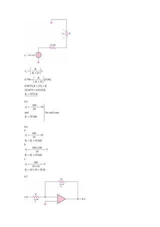
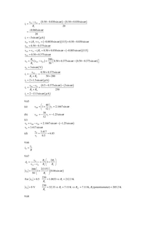
9. ⎛R R R ⎞
vO = − ⎜ F ⋅ vI 1 + F ⋅ vI 2 + F ⋅ vI 3 ⎟
⎝ R1 R2 R3 ⎠
⎡⎛ 100 ⎞ ⎛ 100 ⎞ ⎛ 100 ⎞ ⎤
= − ⎢⎜ ⎟ ( 0.5 ) + ⎜ ⎟ ( 0.75 ) + ⎜ ⎟ ( 2.5 ) ⎥
⎣ ⎝ 50 ⎠ ⎝ 20 ⎠ ⎝ 100 ⎠ ⎦
= − [1 + 3.75 + 2.5]
vO = −7.25 V
(b)
⎡⎛ 100 ⎞ ⎛ 100 ⎞ ⎛ 100 ⎞ ⎤
−2 = − ⎢⎜ ⎟ (1) + ⎜ ⎟ ( 0.8 ) + ⎜ ⎟ vI 3 ⎥
⎣⎝ 50 ⎠ ⎝ 20 ⎠ ⎝ 100 ⎠ ⎦
2 = 2 + 4 + vI 3
vI 3 = −4 V
9.28
− RF R R
vo = ⋅ vI 1 − F ⋅ vI 2 − F ⋅ vI 3
R1 R2 R3
= −4vI 1 − 8vI 2 − 2vI 3
RF RF RF
=4 =8 =2
R1 R2 R3
Largest resistance = RF = 250 K ⇒ R1 = 62.5 K R2 = 31.25 K R3 = 125 K
9.29
RF R
v0 = −4vI 1 − 0.5vI 2 = − vI 1 − F vI 2
R1 R2
RF RF
=4 = 0.5 ⇒ R1 is the smallest resistor
R1 R2
vI 2
i = 100 μ A = = ⇒ R1 = 20 kΩ
R1 R1
⇒ RF = 80 kΩ
⇒ R2 = 160 kΩ
9.30
vI 1 = ( 0.05 ) 2 sin ( 2π ft ) = 0.0707 sin ( 2π ft )
1 1
f = 1 kHz ⇒ T = 3 ⇒ 1 ms vI 2 ⇒ T2 = ⇒ 10 ms
10 100
R R 10 10
vO = − F ⋅ vI 1 − F ⋅ vI 2 = − ⋅ vI 1 − ⋅ vI 2
R1 R2 1 5
vO = − (10 ) ( 0.0707 sin ( 2π ft ) ) − ( 2 )( ±1 V )
vO = −0.707 sin ( 2π ft ) − ( ±2 V )

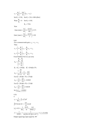
10. 9.31
RF R R
vO = − ⋅ vI 1 − F ⋅ vI 2 − F ⋅ vI 3
R1 R2 R3
20 20 20
vO = − ⋅ vI 1 − ⋅ vI 2 − ⋅ vI 3
10 5 2
K sin ω t = −2vI 1 − 4 [ 2 + 100sin ω t ] − 0
Set vI 1 = −4 mV
9.32
Only two inputs.
⎡R R ⎤
vO = − ⎢ F ⋅ vI 1 + F ⋅ vI 2 ⎥
⎣ R1 R2 ⎦
⎡ 1 ⎤
= − ⎢3vI 1 + ⋅ vI 2 ⎥
⎣ 4 ⎦
RF RF 1
=3 =
R1 R2 4
Smallest resistor = 10 K = R1
RF = 30 K R2 = 120 K
9.33
⎡R R ⎤
vO = − ⎢ F ⋅ vI 1 + F ⋅ vI 2 ⎥
⎣ R1 R2 ⎦
− RF −R R RF
−5 − 5sin ω t = ( 2.5sin ω t ) F ⋅ ( 2 ) ⇒ F = 2 = 2.5
R1 R2 R1 R2
RF = largest resistor ⇒ RF = 200 K
R1 = 100 K R2 = 80 K
9.34
a.
RF R R R
v0 = − ⋅ a3 ( −5 ) − F ⋅ a2 ( −5 ) − F ⋅ a1 ( −5 ) − F ⋅ a0 ( −5 )
R3 R2 R1 R0
RF ⎡ a3 a2 a1 a0 ⎤
So v0 = + + + ( 5)
10 ⎢ 2 4 8 16 ⎥
⎣ ⎦
R 1
b. v0 = 2.5 = F ⋅ ⋅ 5 ⇒ RF = 10 kΩ
10 2
c.
10 1
i. v0 = ⋅ ⋅ 5 ⇒ v0 = 0.3125 V
10 16

11. 10 ⎡ 1 1 1 1 ⎤
ii. v0 = + + + ( 5 ) ⇒ v0 = 4.6875 V
10 ⎢ 2 4 8 16 ⎥
⎣ ⎦
9.35
(a)
10
vO1 = − ⋅ vI 1
1
20 20
vO = − ⋅ vO1 − ⋅ vI 2 = − ( 20 )( −10 ) vI 1 − ( 20 ) vI 2
1 1
vO = 200vI 1 − 20vI 2
(b)
vI 1 = 1 + 2sin ω t ( mV )
vI 2 = −10 mV
Then vO = 200 (1 + 2sin ω t ) − 20 ( −10 )
So vO = 0.4 + 0.4sin ω t (V )
9.36
For one-input
v0
v1 = −
Aod
vI 1 − v1 v1 v −v
= + 1 0
R1 R2 R3 RF
VI 1 ⎡1 1 1 ⎤ v0
= v1 ⎢ + + ⎥−
R1 ⎣ R1 R2 R3 RF ⎦ RF
v0 ⎡1 1 1 ⎤ v0
=− ⎢ + + ⎥−
Aod ⎣ R1 R2 R3 RF ⎦ RF
⎧ 1
⎪ 1 1 ⎛ 1 1 ⎞⎫ ⎪
= −v0 ⎨ + + ⎜ + ⎟⎬
⎪ Aod RF RF Aod ⎝ R1 R2 R3 ⎠ ⎪
⎩ ⎭
v0 ⎧ 1 1 RF ⎫
=− ⎨ +1+ ⋅ ⎬
RF ⎩ Aod Aod R1 R2 R3 ⎭
⎧ ⎫
⎪ ⎪
R ⎪ 1 ⎪
v0 = − F ⋅ vI 1 ⋅ ⎨ ⎬ where RP = R1 R2 R3
R1 ⎪1 + 1 ⎛ RF ⎞ ⎪
1+
⎪ Aod ⎜ RP ⎟ ⎪
⎝ ⎠⎭
⎩
−1 ⎛R R R ⎞
Therefore, for three-inputs v0 = × ⎜ F ⋅ vI 1 + F ⋅ vI 2 + F ⋅ vI 3 ⎟
1 ⎛ RF ⎞ ⎝ R1 R2 R3 ⎠
1+ ⎜1 + ⎟
Aod ⎝ RP ⎠
9.37

12. ⎛ R ⎞ R
Av = 12 = ⎜ 1 + 2 ⎟ ⇒ 2 = 11
⎝ R1 ⎠ R1
v v 0.5
i1 = I ⇒ R1 = I =
R1 i1 0.15
R1 = 3.33 K
R2 = 36.7 K
9.38
⎛ 1 ⎞ ⎛ 1 ⎞
vB = ⎜ ⎟ vI v0 = Aod ⎜ ⎟ vi
⎝ 1 + 500 ⎠ ⎝ 501 ⎠
⎛ 1 ⎞
a. 2.5 = Aod ⎜ ⎟ ( 5 ) ⇒ Aod = 250.5
⎝ 501 ⎠
⎛ 1 ⎞
b. v0 = 5000 ⎜ ⎟ ( 5 ) ⇒ v0 = 49.9 V
⎝ 501 ⎠
9.39
⎛ R ⎞
Av = ⎜ 1 + 2 ⎟
⎝ R1 ⎠
(a) Av = 11
(b) Av = 2
(c) Av = 1.2
(d) Av = 11
(e) Av = 3
(f) Av = 2
9.40
R2
(a) = 1 ⇒ R1 = R2 = 20 K
R1
R2
(b) = 9 ⇒ R1 = 20 K, R2 = 180 K
R1
R2
(c) = 49 ⇒ R1 = 20 K, R2 = 980 K
R1
R2
(d) = 0 can set R2 = 20 K, R1 = ∞ (open circuit)
R1
9.41
⎛ 50 ⎞ ⎡⎛ 20 ⎞ ⎛ 40 ⎞ ⎤
v0 = ⎜ 1 + ⎟ ⎢⎜ ⎟ vI 2 + ⎜ ⎟ vI 1 ⎥
⎝ 50 ⎠ ⎣⎝ 20 + 40 ⎠ ⎝ 20 + 40 ⎠ ⎦
v0 = 1.33vI 1 + 0.667vI 2
9.42
(a)

13. vI 1 − v2 vI 2 − v2 v2
+ =
20 40 10
⎛ 100 ⎞
vO = ⎜ 1 + ⎟ v2 = 3v2
⎝ 50 ⎠
Now 2vI 1 − 2v2 + vI 2 − v2 = 4v2
⎛v ⎞
2vI 1 + vI 2 = 7v2 = 7 ⎜ o ⎟
⎝3⎠
6 3
So vO = ⋅ vI 1 + ⋅ vI 2
7 7
( 0.2 ) + ⎛ ⎞ ( 0.3) ⇒ vO = 0.3 V
6 3
(b) vO = ⎜ ⎟
7 ⎝ 7⎠
⎛6⎞ ⎛ 3⎞
(c) vO = ⎜ ⎟ ( 0.25 ) + ⎜ ⎟ ( −0.4 ) ⇒ vO = 42.86 mV
⎝7⎠ ⎝7⎠
9.43
⎛ R4 ⎞
v2 = ⎜ ⎟ vI
⎝ R3 + R4 ⎠
⎛ R ⎞ ⎛ R ⎞ ⎛ R4 ⎞
vO = ⎜1 + 2 ⎟ v2 = ⎜ 1 + 2 ⎟ ⎜ ⎟ vI
⎝ R1 ⎠ ⎝ R1 ⎠⎝ R3 + R4 ⎠
vO ⎛ R2 ⎞ ⎛ R4 ⎞
Av = = ⎜1 + ⎟ ⎜ ⎟
vI ⎝ R1 ⎠ ⎝ R3 + R4 ⎠
9.44
(a)
vO ⎛ 50 x ⎞
= ⎜1 +
⎜ (1 − x ) 50 ⎟
⎟
vI ⎝ ⎠
vO ⎛ x ⎞ 1− x + x
= ⎜1 + ⎟=
vI ⎝ 1 − x ⎠ 1− x
v 1
Av = O =
vI 1 − x
(b) 1 ≤ Av ≤ ∞
(c) If x = 1, gain goes to infinity.
9.45
Change resister values as shown.

14. vI
i1 = = i2
R
⎛v ⎞
vx = i2 2 R + vI = ⎜ I ⎟ 2 R + vI = 3vI
⎝R⎠
v x 3I
i3 = =
R R
v 3v 4v
i4 = i2 + i3 = I + I = I
R R R
⎛ 4vI ⎞
v0 = i4 2 R + vx = ⎜ ⎟ 2 R + 3vI
⎝ R ⎠
v0
= 11
vI
9.46
vO
(a) =1
vI
(b) From Exercise TYU9.7
⎛ R2 ⎞
⎜1 + ⎟
vO
= ⎝ R1 ⎠
vI ⎡ 1 ⎛ R2 ⎞ ⎤
⎢1 + ⎜1 + ⎟ ⎥
⎣ Aod ⎝ R1 ⎠ ⎦
But R2 = 0, R1 = ∞
vO 1 1 v
= = ⇒ O = 0.999993
vI 1 + 1 1 vI
1+
Aod 1.5 × 105
vO 1
(b) Want = 0.990 = ⇒ Aod = 99
vI 1
1+
Aod
9.47

15. v0 = Aod ( vI − v0 )
⎛ 1 ⎞
⎜ + 1⎟ v0 = vI
⎝ Aod ⎠
v0 1
=
vI ⎛ 1 ⎞
⎜1 + ⎟
⎝ Aod ⎠
v
Aod = 104 ; 0 = 0.99990
vI
v0
Aod = 103 ; = 0.9990
vI
v0
Aod = 102 ; = 0.990
vI
v0
Aod = 10; = 0.909
vI
9.48
⎛ R ⎞
v0 A = ⎜ 1 + 2 ⎟ vI
⎝ R1 ⎠
⎛ R ⎞ ⎛ R ⎞
v01 = ⎜1 + 2 ⎟ vI , v02 = − ⎜ 1 + 2 ⎟ vI
⎝ R1 ⎠ ⎝ R1 ⎠
So v01 = −v02
9.49
vI
(a) iL =
R1
(b)
vO1 = iL RL + vI = iL RL + iL R1
vOI ( max ) ≅ 10 V = iL (1 + 9 ) = 10iL
So iL ( max ) ≅ 1 mA
Then vI ( max ) ≅ iL R1 = (1)( 9 ) ⇒ vI ( max ) ≅ 9 V
9.50
(a)
⎛ 20 ⎞ ⎛ 20 ⎞
vX = ⎜ ⎟ ⋅ vI = ⎜ ⎟ ( 6 ) = 2
⎝ 20 + 40 ⎠ ⎝ 60 ⎠
vO = 2 V
(b) Same as (a)
(c)
⎛ 6 ⎞
vX = ⎜ ⎟ ( 6 ) = 0.666 V
⎝ 6 + 48 ⎠
⎛ 10 ⎞
vO = ⎜ 1 + ⎟ ⋅ v X ⇒ vO = 1.33 V
⎝ 10 ⎠
9.51
a.

16. v1 v −v
Rin = and 1 0 = i1 and v0 = − Aod v1
i1 RF
v1 − ( − Aod v1 ) v1 (1 + Aod )
So i1 = =
RF RF
v1 RF
Then Rin = =
i1 1 + Aod
b.
⎛ RS ⎞ RF
i1 = ⎜ ⎟ iS and v0 = − Aod ⋅ ⋅ i1
⎝ RS + Rin ⎠ 1 + Aod
⎛ A ⎞⎛ RS ⎞
So v0 = − RF ⎜ od ⎟⎜ ⎟ iS
⎝ 1 + Aod ⎠⎝ RS + Rin ⎠
RF 10
Rin = = = 0.009990
1 + Aod 1001
⎛ 1000 ⎞ ⎛ RS ⎞
v0 = − RF ⎜ ⎟⎜ ⎟ iS
⎝ 1001 ⎠ ⎝ RS + 0.009990 ⎠
⎛ 1000 ⎞ ⎛ RS ⎞
Want ⎜ ⎟⎜ ⎟ ≤ 0.990
⎝ 1001 ⎠ ⎝ RS + 0.009990 ⎠
which yields RS ≥ 1.099 kΩ
9.52
vO = iC RF , 0 ≤ iC ≤ 8 mA
For vO ( max ) = 8 V, Then RF = 1 k Ω
9.53
v 10
i = I so 1 = ⇒ R = 10 kΩ
R R
In the ideal op-amp, R1 has no influence.
⎛ R ⎞
Output voltage: v0 = ⎜1 + 2 ⎟ vI
⎝ R⎠
v0 must remain within the bias voltages of the op-amp; the larger the R2, the smaller the range of input
voltage vI in which the output is valid.
9.54
(a)

17. − vI
iL =
R2
− ( −10V )
10mA =
R2
R2 = 1 K
1 R
Also = F
R2 R1 R3
vL = (10mA )( 0.05k ) = 0.5 V
0.5
i2 = = 0.5 mA
1
iR 3 = 10 + 0.5 = 10.5 mA
v −v 13 − 0.5
Limit vo to 13V ⇒ R3 = O L = R3 = 1.19 K
iR 3 10.5
RF R3 1.19 R
Then = = = 1.19 = F
R1 R2 1 R1
For example, RF = 119 K, R1 = 100 K
(b) From part (a), vO = 13 V when vI = −10 V
9.55
(a)
vx
i1 = i2 and i2 = + iD , vx = −i2 RF
R2
⎛R ⎞
Then i1 = −i1 ⎜ F ⎟ + iD
⎝ R2 ⎠
⎛ R ⎞
Or iD = i1 ⎜ 1 + F ⎟
⎝ R2 ⎠
(b)
vI 5
R1 = = ⇒ R1 = 5 k Ω
i1 1
⎛ R ⎞ R
12 = (1) ⎜ 1 + F ⎟ ⇒ F = 11
⎝ R2 ⎠ R2
For example, R2 = 5 k Ω, RF = 55 k Ω
9.56
VX VX − vO
(1) IX = +
R2 R3
VX VX − vO
(2) + =0
R1 RF

18. ⎛ R ⎞
From (2) vO = VX ⎜ 1 + F ⎟
⎝ R1 ⎠
⎛ 1 1 ⎞ 1 ⎛ R ⎞
Then (1) I X = VX ⎜ + ⎟ − ⋅ VX ⎜1 + F ⎟
⎝ R2 R3 ⎠ R3 ⎝ R1 ⎠
IX 1 1 1 1 R 1 R
= = + − − F = − F
VX R0 R2 R3 R3 R1 R3 R2 R1 R3
R1 R3 − R2 RF
=
R1 R2 R3
R1 R2 R3
or Ro =
R1 R3 − R2 RF
RF 1
Note: If = ⇒ R2 RF = R1 R3 then Ro = ∞, which corresponds to an ideal current source.
R1 R3 R2
9.57
R2 R4
Ad = = =5
R1 R3
Minimum resistance seen by vI1 is R1.
Set R1 = R3 = 25 kΩ Then R2 = R4 = 125 kΩ
v0
iL = ⇒ v0 = iL RL = ( 0.5 )( 5 ) = 2.5 V
RL
v0 = 5 ( vI 2 − vI 1 )
2.5 = 5 ( vI 2 − 2 ) ⇒ vI 2 = 2.5 V
9.58
R2
vO = ( vI 2 − vI 1 )
R1
R2 R R
Ad = and 2 = 4 with R2 = R4 and R1 = R3
R1 R1 R3
Differential input resistance
R 20
Ri = 2 R1 ⇒ R1 = i = = 10 K
2 2
R2
(a) = 50 ⇒ R2 = R4 = 500 K
R1
R1 = R3 = 10 K
R2
(b) = 20 ⇒ R2 = R4 = 200 K
R1
R1 = R3 = 10 K
R2
(c) = 2 ⇒ R2 = R4 = 20 K
R1
R1 = R3 = 10 K
R2
(d) = 0.5 ⇒ R2 = R4 = 5 K
R1
R1 = R3 = 10 K
9.59

19. We have
⎛ R ⎞⎛ R / R ⎞ ⎛R ⎞ ⎛ R ⎞⎛ 1 ⎞ ⎛ R2 ⎞
vO = ⎜ 1 + 2 ⎟ ⎜ 4 3 ⎟ vI 2 − ⎜ 2 ⎟ vI 1 or vO = ⎜ 1 + 2 ⎟ ⎜ ⎟ vI 2 − ⎜ ⎟ vI 1
⎝ R1 ⎠ ⎝ 1 + R4 / R3 ⎠ ⎝ R1 ⎠ ⎝ R1 ⎠ ⎝ 1 + R3 / R4 ⎠ ⎝ R1 ⎠
Set R2 = 50 (1 + x ) , R1 = 50 (1 − x )
R3 = 50 (1 − x ) , R4 = 50 (1 + x )
⎡ ⎤
⎡ ⎛ 1 + x ⎞⎤ ⎢ ⎥ 1+ x ⎞
⎥ vI 2 − ⎛
1
vO = ⎢1 + ⎜ ⎟⎥ ⎢ ⎜ ⎟ vI 1
⎣ ⎝ 1 − x ⎠ ⎦ ⎢1 + ⎛ 1 − x ⎞ ⎥ ⎝ 1− x ⎠
⎢ ⎜ 1+ x ⎟ ⎥
⎣ ⎝ ⎠⎦
⎡1 − x + (1 + x ) ⎤ ⎡ 1+ x ⎤ ⎛ 1+ x ⎞
vO = ⎢ ⎥⋅⎢ ⎥ vI 2 − ⎜ ⎟ vI 1
⎣ 1− x ⎦ ⎢1 + x + (1 − x ) ⎥
⎣ ⎦ ⎝ 1− x ⎠
⎛ 1+ x ⎞ ⎛1+ x ⎞
=⎜ ⎟ vI 2 − ⎜ ⎟ vI 1
⎝1− x ⎠ ⎝ 1− x ⎠
For vI 1 = vI 2 ⇒ vO = 0
Set R2 = 50 (1 + x ) R1 = 50 (1 − x )
R3 = 50 (1 + x ) R4 = 50 (1 − x )
⎛ ⎞
⎛ 1+ x ⎞⎜ 1 ⎟ ⎛ 1+ x ⎞
vO = ⎜1 + ⎟ ⎜ 1 + x ⎟ vI 2 − ⎜ ⎟ vI 1
⎝ 1− x ⎠⎜1+ ⎟ ⎝ 1− x ⎠
⎜ ⎟
⎝ 1− x ⎠
⎛ 1+ x ⎞
= vI 2 − ⎜ ⎟ vI 1
⎝ 1− x ⎠
vI 1 = vI 2 = vcm
vO 1 + x 1 − x − (1 + x ) −2 x
= 1− = =
vcm 1− x 1− x 1− x
Set R2 = 50 (1 − x ) R1 = 50 (1 + x )
R3 = 50 (1 − x ) R4 = 50 (1 + x )
⎛ ⎞
⎛ 1− x ⎞⎜ 1 ⎟ ⎛ 1− x ⎞
vO = ⎜ 1 + ⎟ ⎜ 1 − x ⎟ vI 2 − ⎜ ⎟ vI 1
⎝ 1+ x ⎠⎜ 1+ ⎟ ⎝ 1+ x ⎠
⎜ ⎟
⎝ 1+ x ⎠
⎛ 1− x ⎞
= ⎜1 − ⎟ vcm
⎝ 1+ x ⎠
1 + x − (1 − x )
2x
Acm = =
1+ x 1+ x
Worst common-mode gain
−2 x
Acm =
1− x
(b)

20. −2 x −2 ( 0.01)
For x = 0.01, Acm = = = −0.0202
1 − x 1 − 0.01
−2 ( 0.02 )
For x = 0.02, Acm = = −0.04082
1 − 0.02
−2 ( 0.05 )
For x = 0.05, Acm = = −0.1053
1 − 0.05
1 1
For this condition, set vI 2 = + , vI 1 = − ⇒ vd = 1 V
2 2
1 ⎡ ⎛ 1 + x ⎞ ⎤ 1 ⎡1 − x + (1 + x ) ⎤ 1 2 1
Ad = ⎢1 + ⎜ ⎟⎥ = ⎢ ⎥= ⋅ =
2 ⎣ ⎝ 1 − x ⎠⎦ 2 ⎣ 1− x ⎦ 2 1− x 1− x
1.010
For x = 0.01 Ad = 1.010 C M R RdB = 20 log10 = 33.98 dB
0.0202
1 1.020
For x = 0.02, Ad = = 1.020 C M R RdB = 20 log10 = 27.96 dB
0.98 0.04082
1 1.0526
For x = 0.05 Ad = = 1.0526 C M R RdB = 20 log10 ≅ 20 dB
0.95 0.1053
9.60
⎛ 10R ⎞ ⎛ 10 ⎞
vy = ⎜ ⎟ v2 = ⎜ ⎟ ( 2.65 ) ⇒ v y = vx = 2.40909 V
⎝ 10R+R ⎠ ⎝ 11 ⎠
v2 − v y 2.65 − 2.40909
i3 = i4 = = = 0.0120 mA
R 20
v −v 2.50 − 2.40909
i1 = i2 = 1 x = = 0.0045455 mA
R 20
vO = vx − i2 (10R ) = ( 2.40909 ) − ( 0.0045455 )( 200 )
vO = 1.50 V
9.61
10
iE = (1 + β )( iB ) = ( 81)( 2 ) = 162 mA =
R
R = 61.73 Ω
9.62
a. From superposition:
R2
v01 = − ⋅ vI 1
R1
⎛ R ⎞ ⎛ R1 ⎞
v02 = ⎜ 1 + 2 ⎟ ⎜ ⎟ vI 2
⎝ R1 ⎠ ⎝ R3 + R4 ⎠
Setting vI 1 = vI 2 = vcm
⎡ ⎛ ⎞ ⎤
⎢⎛ R ⎞ ⎜ 1 ⎟ R ⎥
v0 = v01 + v02 = ⎢⎜ 1 + 2 ⎟ ⎜ ⎟ − 2 ⎥ vcm
⎢⎝ R1 ⎠ ⎜ R3 ⎟ R1 ⎥
⎢ ⎜ 1+ R ⎟ ⎥
⎣ ⎝ 4 ⎠ ⎦

21. ⎛ ⎞
v R ⎛ R ⎞⎜ 1 ⎟ R
Acm = 0 = 4 ⋅ ⎜ 1 + 2 ⎟ ⎜ ⎟− 2
vcm R3 ⎝ R1 ⎠ ⎜ R4 ⎟ R1
⎜ 1+ R ⎟
⎝ 3 ⎠
R4 ⎛ R2 ⎞ R2 ⎛ R4 ⎞
⎜1 + ⎟ − ⎜1 + ⎟
= 3⎝
R R1 ⎠ R1 ⎝ R3 ⎠
⎛ R4 ⎞
⎜1 + ⎟
⎝ R3 ⎠
R4 R2
−
R R1
Acm = 3
⎛ R4 ⎞
⎜1 + ⎟
⎝ R3 ⎠
R4 R
b. Max. Acm ⇒ Min. and Max. 2
R3 R1
47.5 52.5
−
Max. Acm = 10.5 9.5 = 4.5238 − 5.5263 ⇒ A = 0.1815
1 + 4.5238
cm
47.5 max
1+
10.5
9.63
vI 1 − v A v A − vB vA − v0
= + (1)
R1 + R2 Rv R2
vI 2 − vB vB − v A vB
= + (2)
R1 + R2 Rv R2
⎛ R1 ⎞ ⎛ R2 ⎞
v− = ⎜ ⎟ vA + ⎜ ⎟ vI 1 (3)
⎝ R1 + R2 ⎠ ⎝ R1 + R2 ⎠
⎛ R1 ⎞ ⎛ R2 ⎞
v+ = ⎜ ⎟ vB + ⎜ ⎟ vI 2 (4)
⎝ R1 + R2 ⎠ ⎝ R1 + R2 ⎠

22. Now v− = v+ ⇒ R1vA + R2 vI 1 = R1vB + R2 vI 2
R
So that v A = vB + 2 ( vI 2 − vI 1 )
R1
vI 1 ⎛ 1 1 1 ⎞ v v
= vA ⎜ + + ⎟− B − 0 (1)
R1 + R2 ⎝ R1 + R2 RV R2 ⎠ RV R2
vI 2 ⎛ 1 1 1 ⎞ v
= vB ⎜ + + ⎟− A ( 2)
R1 + R2 ⎝ R1 + R2 RV R2 ⎠ RV
Then
vI 1 ⎛ 1 1 1 ⎞ v v ⎛ R ⎞⎛ 1 1 1 ⎞
= vB ⎜ + + ⎟ − B − 0 + ⎜ 2 ⎟⎜ + + ⎟ ( vI 2 − vI 1 ) (1)
R1 + R2 ⎝ R1 + R2 RV R2 ⎠ RV R2 ⎝ R1 ⎠ ⎝ R1 + R2 RV R2 ⎠
vI 2 ⎛ 1 1 1 ⎞ 1 ⎡ R2 ⎤
= vB ⎜ + + ⎟− ⎢ vB + ( vI 2 − vI 1 ) ⎥ (2)
R1 + R2 ⎝ R1 + R2 RV R2 ⎠ RV ⎣ R1 ⎦
Subtract (2) from (1)
1 ⎛ R ⎞⎛ 1 1 1 ⎞ v 1 R2
( vI 1 − vI 2 ) = ⎜ 2 ⎟ ⎜ + + ⎟ ( vI 2 − vI 1 ) − 0 + ⋅ ( vI 2 − vI 1 )
R1 + R2 ⎝ R1 ⎠ ⎝ R1 + R2 RV R2 ⎠ R2 RV R1
v0 ⎧⎛ R ⎞ ⎛ 1
⎪ 1 1 ⎞ 1 ⎫
1 R2 ⎪
= ( vI 2 − vI 1 ) ⎨⎜ 2 ⎟ ⎜ + + ⎟+ + ⋅ ⎬
R2 ⎪⎝ R1 ⎠ ⎝ R1 + R2 RV R2 ⎠ R1 + R2 RV R1 ⎪
⎩ ⎭
⎛ R ⎞ ⎧ R2 R R1 R ⎫
v0 = ( vI 2 − vI 1 ) ⎜ 2 ⎟ ⎨ + 2 +1+ + 2⎬
⎝ R1 ⎠ ⎩ R1 + R2 RV R1 + R2 RV ⎭
2 R2 ⎛ R2 ⎞
v0 = ⎜1 + ⎟ ( vI 2 − vI 1 )
R1 ⎝ RV ⎠
9.64

23. vI 1 − vI 2 ( 0.50 − 0.030sin ω t ) − ( 0.50 + 0.030sin ω t )
i1 = =
R1 20
−0.060sin ω t
=
20
i1 = −3sin ω t ( μ A )
vO1 = i1 R2 + vI 1 = ( −0.0030sin ω t )(115 ) + 0.50 − 0.030sin ω t
vO1 = 0.50 − 0.375sin ω t
vO 2 = vI 2 − i1 R2 = 0.50 + 0.030sin ω t − ( −0.003sin ω t )(115 )
vO 2 = 0.50 + 0.375sin ω t
R4 200
vO = ( vO 2 − vO1 ) = ⎡ 0.50 + 0.375sin ω t − ( 0.50 − 0.375sin ω t ) ⎤
R3 50 ⎣ ⎦
vO = 3sin ω t ( V )
vO 2 0.50 + 0.375sin ω t
i3 = =
R3 + R4 50 + 200
i3 = 2 + 1.5sin ω t ( μ A )
vO1 − vO ( 0.5 − 0.375sin ω t ) − ( 3sin ω t )
i2 = =
R3 + R4 250
i2 = 2 − 13.5sin ω t ( μ A )
9.65
⎛ 40 ⎞
(a) vOB = ⎜1 + ⎟ vI = 2.1667 sin ω t
⎝ 12 ⎠
30
(b) vOC = − vI = −1.25sin ω t
12
(c)
vO = vOB − vOC = 2.1667 sin ω t − ( −1.25sin ω t )
vO = 3.417 sin ω t
vO 3.417
(d) = = 6.83
vI 0.5
9.66
vI
iO =
R
9.67
vO R ⎛ 2R ⎞
Ad = = 4 ⎜1 + 2 ⎟
vI 2 − vI 1 R3 ⎝ R1 ⎠
200 ⎛ 2 (115 ) ⎞
vO = ⎜1 + ⎟ ( 0.06sin ω t )
50 ⎝ R1 ⎠
230
For vO = 0.5 = 1.0833 ⇒ R1 = 212.3 K
R1
230
vO = 8 V = 32.33 ⇒ R1 = 7.11 K ⇒ R1 f = 7.11 K, R1 (potentiometer) = 205.2 K
R1
9.68

24. ⎛ 2 R2 ⎞
R4
vO = ⎜1 + ⎟ ( vI 2 − vI 1 )
⎝
R3 R1 ⎠
Set R2 = 15 K, Set R1 = 2 K + 100 k ( Rot )
R4
Want ≈8 Set R3 = 10 K
R3
R 4 = 75 K
Now
75 ⎛ 2 (15 ) ⎞
Gain (min) = ⎜1 + ⎟ = 9.71
10 ⎝ 102 ⎠
75 ⎛ 2 (15 ) ⎞
Gain ( max ) = ⎜1 + ⎟ = 120
10 ⎝ 2 ⎠
9.69
For a common-mode gain, vcm = vI 1 = vI 2
Then
⎛ R ⎞ R
v01 = ⎜ 1 + 2 ⎟ vcm − 2 vcm = vcm
⎝ R1 ⎠ R1
⎛ R ⎞ R
v02 = ⎜ 1 + 2 ⎟ vcm − 2 vcm = vcm
⎝ R1 ⎠ R1
From Problem 9.62 we can write
R4 R4
−
R3 R3 ′
Acm =
⎛ R4 ⎞
⎜1 + ⎟
⎝ R3 ⎠
′
R3 = R4 = 20 kΩ, R3 = 20 kΩ ± 5%
20
1−
R3 1 ⎛ 20 ⎞
′
Acm = = ⎜1 − ⎟
(1 + 1) 2 ⎝ ′
R3 ⎠
′
For R3 = 20 kΩ − 5% = 19 kΩ
1 ⎛ 20 ⎞
Acm = ⎜ 1 − ⎟ = −0.0263
2 ⎝ 19 ⎠
′
For R3 = 20 kΩ + 5% = 21 kΩ
1 ⎛ 20 ⎞
Acm = ⎜ 1 − ⎟ = 0.0238
2⎝ 21 ⎠
So Acm max = 0.0263
9.70
a.
1
⋅ vI ( t ′ ) dt ′
R1C2 ∫
v0 =
0.5
∫ 0.5sin ω t dt = − ω cos ω t
1 ( 0.5 ) 0.5
v0 = 0.5 = ⋅ =
R1C2 ω 2π R1C2 f
1 1
f = = ⇒ f = 31.8 Hz
2π R1C2 2π ( 50 × 103 )( 0.1× 10−6 )
Output signal lags input signal by 90°

25. b.
0.5
i. f = ⇒ f = 15.9 Hz
2π ( 50 × 103 )( 0.1× 10−6 )
0.5
ii. f = ⇒ f = 159 Hz
( 0.1)( 2π ) ( 50 ×103 )( 0.1×10−6 )
9.71
1 − vI ⋅ t
vO = −
RC ∫ vI ( t ) dt = RC
vI = −0.2
Now
− ( −0.2 )( 2 )
8=
RC
(a) RC = 0.05 s
( 0.2 ) t
(b) 14 = ⇒ t = 3.5 s
0.05
9.72
a.
1 1
− R2 R2 ⋅
v0 jω C2 jω C2
= =−
vI R1 ⎛ 1 ⎞
R1 ⎜ R2 + ⎟
⎝ jω C2 ⎠
v0 R 1
=− 2⋅
vI R1 1 + jω R2 C2
v0 R
b. =− 2
vI R1
1
c. f =
2π R2 C2
9.73
a.
v0 − R2 R ( jω C1 )
= =− 2
vI R + 1 1 + jω R1C1
jω C1
1
v0 R jω R1C1
=− 2⋅
vI R1 1 + jω R1C1
v0 R
b. =− 2
vI R1
1
c. f =
2π R1C1
9.74
Assuming the Zener diode is in breakdown,

26. R2 1
vO = − ⋅ Vz = − ( 6.8 ) ⇒ vO = −6.8 V
R1 1
0 − vO 0 − ( −6.8 )
i2 = = ⇒ i2 = 6.8 mA
R2 1
10 − Vz 10 − 6.8
iz = − i2 = − 6.8 ⇒ iz = −6.2 mA!!!
Rs 5.6
Circuit is not in breakdown. Now
10 − 0 10
= i2 = ⇒ i2 = 1.52 mA
Rs + R1 5.6 + 1
vO = −i2 R2 = − (1.52 )(1) ⇒ vO = −1.52 V
iz = 0
9.75
⎛ v ⎞ ⎡ v ⎤ ⎛ vI ⎞
vO = −VT ln ⎜ I ⎟ = − ( 0.026 ) ln ⎢ −14 I 4 ⎥ ⇒ vO = −0.026 ln ⎜ −10 ⎟
⎝ I s R1 ⎠ ⎢ (10 )(10 ) ⎥
⎣ ⎦ ⎝ 10 ⎠
For vI = 20 mV , vO = 0.497 V
For vI = 2 V , vO = 0.617 V
9.76

27. ⎛ 333 ⎞
v0 = ⎜ ⎟ ( v01 − v02 ) = 16.65 ( v01 − v02 )
⎝ 20 ⎠
⎛i ⎞
v01 = −vBE1 = −VT ln ⎜ C1 ⎟
⎝ IS ⎠
⎛i ⎞
v02 = −vBE 2 = −VT ln ⎜ C 2 ⎟
⎝ IS ⎠
⎛i ⎞ ⎛i ⎞
v01 − v02 = −VT ln ⎜ C1 ⎟ = VT ln ⎜ C 2 ⎟
⎝ iC 2 ⎠ ⎝ iC1 ⎠
v v
iC 2 = 2 , iC1 = 1
R2 R1
⎛v R ⎞
So v01 − v02 = VT ln ⎜ 2 ⋅ 1 ⎟
⎝ R2 v1 ⎠
Then
⎛v R ⎞
v0 = (16.65 )( 0.026 ) ln ⎜ 2 ⋅ 1 ⎟
⎝ v1 R2 ⎠
⎛v R ⎞
v0 = 0.4329 ln ⎜ 2 ⋅ 1 ⎟
⎝ v1 R2 ⎠
ln ( x ) = log e ( x ) = ⎡ log10 ( x ) ⎤ ⋅ ⎡log e (10 ) ⎤
⎣ ⎦ ⎣ ⎦
= 2.3026 log10 ( x )
⎛v R ⎞
Then v0 ≅ (1.0 ) log10 ⎜ 2 ⋅ 1 ⎟
⎝ v1 R2 ⎠
9.77
( )
vO = − I s R evI / VT = − (10−14 )(104 ) evI / VT
vO = (10 −10
)e vI / 0.026
For vI = 0.30 V , vo = 1.03 × 10−5 V
For vI = 0.60 V , vo = 1.05 V