1. Chapter 9
Exercise Solutions
EX9.1
R2
Av = −15 = −
R1
R1 = Ri = 20 K ⇒ R2 = 15 R1 = 15 ( 20 ) = 300 K
EX9.2
R2 ⎛ R3 ⎞ R3
We can write ACL = − ⎜1 + ⎟ −
R1 ⎝ R4 ⎠ R1
R1 = R1 = 10 kΩ
Want ACL = −50 Set R2 = R3 = 50 kΩ
⎛ R ⎞
ACL = −50 = −5 ⎜ 1 + 3 ⎟ − 5
⎝ R4 ⎠
R R 50
1+ 3 = 9 ⇒ 3 = 8 =
R4 R4 R4
R4 = 6.25 kΩ
EX9.3
R2 1
We have ACL = − ⋅
R1 ⎡ 1 ⎛ R2 ⎞ ⎤
⎢1 + ⎜1 + ⎟ ⎥
⎣ Ad ⎝ R1 ⎠ ⎦
R
Ri = R1 = 25 kΩ Let 2 = x
R1
x
−12 = −
1
1+ (1 + x )
5 × 103
−x
=
x
1.0002 +
5 × 103
⎛ x ⎞
12 ⎜ 1.0002 + ⎟=x
⎝ 5 × 103 ⎠
12.0024 = x − ( 2.4 × 10 −3 ) x
12.0024 R2
x= = 12.0313 =
0.9976 25 kΩ
R2 = 300.78 kΩ
EX9.4
⎛R R R R ⎞
v0 = − ⎜ F vI 1 + F vI 2 + F vI 3 + F VI 4 ⎟
⎝ R1 R2 R3 R4 ⎠

2. RF R R R
We need = 7, F = 14, F = 3.5, F = 10
R1 R2 R3 R4
Set RF = 280 kΩ
280
Then R1 = = 40 kΩ
7
280
R2 = = 20 kΩ
14
280
R3 = = 80 kΩ
3.5
280
R4 = = 28 kΩ
10
EX9.5
R3 3 R 20 R R
We may note that = = 2 and F = = 2 so that 3 = F
R2 1.5 R1 10 R2 R1
Then
− vI − ( −3)
iL = = ⇒ iL = 2 mA
R2 1.5 kΩ
vL = iL Z L = ( 2 × 10−3 ) ( 200 ) = 0.4 V
vL 0.4
i4 = = = 0.267 mA
R2 1.5 kΩ
i3 = i4 + iL = 0.267 + 2 = 2.267 mA
v0 = i3 R3 + vL = ( 2.267 × 10−3 )( 3 × 103 ) − 0.4 ⇒ v0 = 7.2 V
EX9.6
Refer to Fig. 9.24
R1 = 2 R1 = 5 kΩ
Let R1 = R3 = 2.5 kΩ
Set R2 = R4
v0 R2 R2
Differential Gain = = = 100 = ⇒ R2 = R4 = 250 kΩ
v1 R1 2.5 kΩ
EX9.7

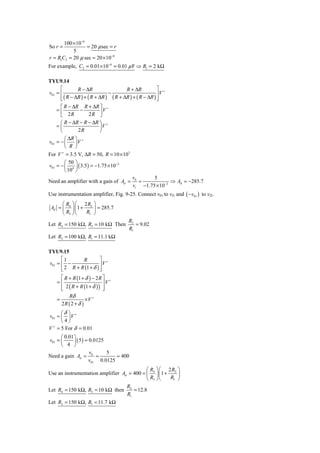
3. We have the general relation that
⎛ R ⎞ ⎛ [ R4 / R3 ] ⎞ R
v0 = ⎜ 1 + 2 ⎟ ⎜ v − 2v
⎜ 1 + [ R / R ] ⎟ I 2 R I1
⎟
⎝ R1 ⎠ ⎝ 4 3 ⎠ 1
R1 = R3 = 10 kΩ, R2 = 20 kΩ, R4 = 21 kΩ
⎛ 20 ⎞ ⎛ [ 21/10] ⎞ ⎛ 20 ⎞
v0 = ⎜ 1 + ⎟ ⎜ ⎟ vI 2 − ⎜ ⎟ vI 1
⎝ 10 ⎠ ⎜ 1 + [ 21/10] ⎟
⎝ ⎠ ⎝ 10 ⎠
v0 = 2.0323vI 2 − 2.0vI
a. vI 1 = 1, vI 2 = −1
v0 = −2.0323 − 2.0 ⇒ v0 = −4.032 V
b. vI 1 = vI 2 = 1 V
v0 = 2.0323 − 2.0 ⇒ v0 = 0.0323 V
c. vcm = vI 1 = vI 2 so common-mode gain
v0
Acm = = 0.0323
vcm
d.
⎛ A ⎞
C M R RdB = 20 log10 ⎜ d ⎟
⎝ Acm ⎠
2.0323 ⎛ 1⎞
Ad = − ( 2.0 ) ⎜ − ⎟ = 2.016
2 ⎝ 2⎠
⎛ 2.016 ⎞
C M R RdB = 20 log10 ⎜ ⎟ = 35.9 d B
⎝ 0.0323 ⎠
EX9.8
R4 ⎛ 2 R2 ⎞
v0 = − ⎜1 + ⎟ ( vI 1 − vI 2 )
R3 ⎝ R1 ⎠
R4 ⎛ 2 R2 ⎞
Differential gain (magnitude) = ⎜1 + ⎟
R3 ⎝ R1 ⎠
Minimum Gain ⇒ Maximum R1 = 1 + 50 = 51 kΩ
20 ⎛ 2 (100 ) ⎞
So Ad = ⎜1 + ⎟ ⇒ Ad = 4.92
20 ⎝ 51 ⎠
Maximum Gain ⇒ Minimum R1 = 1 kΩ
20 ⎛ 2 (100 ) ⎞
Ad = ⎜1 + ⎟ ⇒ Ad = 201
20 ⎝ 1 ⎠
Range of Differential Gain = 4.92 − 201
EX9.9
Time constant = r = R1C2 = (104 )( 0.1×10−6 )
= 1 m sec
−1
0 ≤ t ≤ 1 ⇒ v0 = ×t
R1 C2
At t = 1 m sec ⇒ v0 = −1 V
1
0 ≤ t ≤ 2 ⇒ v0 = −1 + × ( t − 1)
R1 C2
( 2 − 1)
At t = 2 m sec ⇒ v0 = −1 + =0
1

4. EX9.10
v0 = vI 1 + 10vI 2 − 25vI 3 − 80vI 4
From Figure 9.40, v13 input to R1, vI4 input to R2, vI1 input to RA, and vI2 input to RB.
From Equation (9.94)
RF R
= 25 and F = 80
R1 R2
Set RF = 500 kΩ, then R1 = 20 kΩ, and R2 = 6.25 kΩ.
⎛ R ⎞⎛ R ⎞ ⎛ R ⎞⎛ R ⎞
Also ⎜1 + F ⎟⎜ P ⎟ = 1 and ⎜1 + F ⎟ ⎜ P ⎟ = 10
⎝ RN ⎠ ⎝ RA ⎠ ⎝ RN ⎠ ⎝ RB ⎠
where RN = R1 R2 = 20 6.25 = 4.76 kΩ and RP = RA RB RC
RA
We find that = 10
RB
Let RA = 200 kΩ, RB = 20 kΩ
⎛ 500 ⎞ ⎛ RP ⎞ ⎛ RP ⎞
Now ⎜1 + ⎟⎜ ⎟ = 1 = (106 ) ⎜ ⎟
⎝ 4.76 ⎠ ⎝ RA ⎠ ⎝ 200 ⎠
Then RP = 1.89 kΩ
RA RB = 200 20 = 18.2 kΩ
18.2 RC
So RP = 1.89 = ⇒ RC = 2.11 kΩ
18.2 + RC
EX9.11 Computer Analysis
TYU9.1
R2 −100 kΩ
ACL = − = ⇒ ACL = −10
R1 10 kΩ
vI = 0.25 V ⇒ vo = −2.5 V
vI 0.25
i1 = = = 0.025 mA ⇒ i1 = 25 μ A
R1 10 kΩ
i2 = i1 = 25 μ A
Ri = R1 = 10 kΩ
TYU9.2
(a)
− R2
Av =
R1 + RS
−100
Av ( min ) = = −4.926
19 + 1.3
−100
Av ( max ) = = −5.076
19 + 0.7
so 4.926 ≤ Av ≤ 5.076
(b)

5. 0.1
i1 ( max ) = = 5.076 μ A
19 + 0.7
0.1
i1 ( min ) = = 4.926 μ A
19 + 1.3
so 4.926 ≤ i1 ≤ 5.076 μ A
(c) Maximum current specification is violated.
TYU9.3
v0 = Ad ( v2 − v1 ) Ad = 103
a.
v2 = 0, v0 = 5
v 5
v1 = − 0 = − 3 ⇒ v1 = −5 mV
Ad 10
b.
v1 = 5, v0 = −10
v0
= v2 − v1
Ad
−10
= v2 − 5 ⇒ v2 = 4.99 V
103
c.
v1 = 0.001, v2 = −0.001
v0 = 103 ( −0.001 − 0.001)
v0 = −2 V
d.
v2 = 3, v0 = 3
v0 = Ad ( v2 − v1 )
v0
= v2 − v1
Ad
3
= 3 − v1 ⇒ v1 = 2.997 V
103
TYU9.4
⎛R R R ⎞
v0 = − ⎜ 4 vI 1 + 4 vI 2 + 4 vI 3 ⎟
⎝ R1 R2 R3 ⎠
⎡⎛ 40 ⎞ ⎛ 40 ⎞ ⎛ 40 ⎞ ⎤
v0 = − ⎢⎜ ⎟ ( 250 ) + ⎜ ⎟ ( 200 ) + ⎜ ⎟ ( 75 ) ⎥
⎣⎝ 10 ⎠ ⎝ 20 ⎠ ⎝ 30 ⎠ ⎦
v0 = − [1000 + 400 + 100]
v0 = −1500 μ V = −1.5 mV
TYU9.5

6. vI 1 + vI 2 + vI 3 RF
vO = = ( vI 1 + vI 2 + vI 3 )
3 R
RF 1
= ⇒ R1 = R2 = R3 ≡ R = 1 M Ω
R 3
1
Then RF = M Ω = 333 k Ω
3
TYU9.6
v ⎛ R ⎞ R
Av = 0 = ⎜ 1 + 2 ⎟ = 5 so that 2 = 4
vI ⎝ R1 ⎠ R1
For v0 = 10 V, vI = 2 V
2
Then i1 = = 50 μ A ⇒ R1 = 40 kΩ
R1
v0 − vI 10 − 2
Then R2 = 160 kΩ we find i2 = = = 50 μ A
R2 160
TYU9.7
v0 = Aod ( v2 − v1 ) = Aod ( vI − v1 )
v0 v
− vI = −v1 or v1 = vI − 0
Aod Aod
v1 v −v
i1 = = i2 and i2 = 0 1
R1 R2
⎛ 1 ⎞ v −v
Then v1 ⎜ ⎟ = 0 1
⎝ R1 ⎠ R2
⎛ 1 1 ⎞ v
v1 ⎜ + ⎟ = 0
⎝ R1 R2 ⎠ R2
⎛ R ⎞ ⎛ R ⎞⎛ v ⎞
v0 ⎜ 1 + 2 ⎟ v1 = ⎜ 1 + 2 ⎟ ⎜ vI − 0 ⎟
⎝ R1 ⎠ ⎝ R1 ⎠⎝ Aod ⎠
⎛ R2 ⎞
⎜1 + ⎟
So Av = =
v0 ⎝ R1 ⎠
vI 1 ⎛ R2 ⎞
1+ ⎜1 + ⎟
Aod ⎝ R1 ⎠
TYU9.8

7. ⎛ Rb ⎞
For vI 2 = 0, v2 = ⎜ ⎟ vI 1 and
⎝ Rb + Ra ⎠
⎛ R ⎞ ⎛ Rb ⎞
v0 ( vI 1 ) = ⎜ 1 + 2 ⎟ ⎜ ⎟ vI 1
⎝ R1 ⎠⎝ Rb + Ra ⎠
⎛ 70 ⎞⎛ 50 ⎞
= ⎜ 1 + ⎟⎜ ⎟ vI 1
⎝ 5 ⎠⎝ 50 + 25 ⎠
= 10vI 1
⎛ Ra ⎞
For vI 1 = 0, v2 = ⎜ ⎟ vI 2
⎝ Rb + Ra ⎠
⎛ R ⎞ ⎛ Ra ⎞
v0 ( vI 2 ) = ⎜ 1 + 2 ⎟ ⎜ ⎟ vI 2
⎝ R1 ⎠⎝ Rb + Ra ⎠
⎛ 70 ⎞⎛ 25 ⎞
= ⎜ 1 + ⎟⎜ ⎟ vI 2
⎝ 5 ⎠⎝ 25 + 50 ⎠
= 5vI 2
Then
v0 = v0 ( vI 1 ) + v0 ( vI 2 )
v0 = 10vI 1 + 5vI 2
TYU9.9
RS Ri so i1 = i2 = iS = 100 μ A
v0 = −iS RF
We want −10 = − (100 × 10−6 ) RF ⇒ RF = 100 kΩ
TYU9.10
We want iL = 1 mA when vI = −5 V
−VI −v − ( −5 )
iL = ⇒ R2 = I = ⇒ R2 = 5 kΩ
R2 i2 10−3
vL = iL Z L = (10−3 ) ( 500 ) ⇒ vL = 0.5 V
vL 0.5
i4 = = ⇒ i4 = 0.1 mA
R2 5 kΩ
i3 = i4 + iL = 0.1 + 1 = 1.1 mA
If op-amp is biased at ±10 V, output must be limited to ≈ 8 V.
So v0 = i3 R3 + vL
8 = (1.1× 10−3 ) R3 + 0.5 ⇒ R3 = 6.82 kΩ
Let R3 = 7.0 kΩ

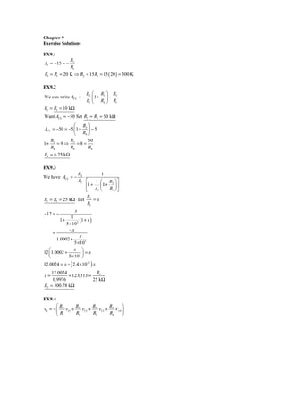
8. R3 RF 7
Then we want = = = 1.4
R2 R1 5
Can choose R1 = 10 kΩ and RF = 14 kΩ
TYU9.11
a.
v −v
i1 = I 1 I 2
R1
R4
′
v01 = vI 1 + i1 R2 , v02 = vI 2 − i1 R2 and v0 = ( v02 − v01 )
R3
R4
v0 = [vI 2 − i1 R2 − vI 1 − i1 R2′ ]
R3
R4
v0 = ⎡( vI 2 − vI 1 ) − i1 ( R2 + R2 ) ⎤
′ ⎦
R3 ⎣
R4 ⎡ ⎛ vI 2 − vI 1 ⎞ ⎤
v0 = ⎢ ( vI 2 − vI 1 ) − ⎜ ⎟ ( R2 + R2 ) ⎥
′
R3 ⎣ ⎝ R1 ⎠ ⎦
For common-mode input vI 2 = vI 1 ⇒ v0 = 0 ⇒ Common Gain = 0, C M R R = ∞
b. Ad ( min ) ⇒ R2 min, R1 max
′
⎛ 20 ⎞ ⎡ 100 + 95 ⎤
Ad = ⎜ ⎟ ⎢1 + ⎥ = 4.82
⎝ 20 ⎠ ⎣ 51 ⎦
⎛ 20 ⎞ ⎡ 100 + 105 ⎤
Ad ( max ) = ⎜ ⎟ ⎢1 + ⎥ = 206
⎝ 20 ⎠ ⎣ 1 ⎦
c.
A
CM RR = d
Acm
Acm = 0 ⇒ C M R R = ∞
TYU9.12
R4 ⎛ 2 R2 ⎞
Differential Gain = ⎜1 + ⎟
R3 ⎝ R1 ⎠
Let R3 = R4 so the difference amplifier gain is unity.
Minimum Gain ⇒ Maximum R1
⎛ 2 R2 ⎞
So ⎜1 +
⎜ R ( max ) ⎟ = 2
⎟
⎝ 1 ⎠
We want 2 R2 = R1 ( max )
Maximum Gain ⇒ Minimum R1
⎛ 2 R2 ⎞
⎜ R ( min ) ⎟ = 1000 or 2 R2 = 999 R1 ( min )
So ⎜1 + ⎟
⎝ 1 ⎠
If R2 = 50 kΩ, let R1 ( min ) = 100 Ω fixed resistor and let R1 ( max ) = 100 kΩ + 100 Ω = 100.1
pot
Then actual differential gain is in the range of 1.999 − 1001
TYU9.13
−1 10 μ sec −10 × 10−6
End of 1st pulse: v0 = ×t 0 =
r r
− (10 ) (10 × 10−6 )
After 10 pulses: v0 = −5 =
r

9. 100 × 10−6
So r = = 20 μ sec = r
5
r = R1C2 = 20 μ sec = 20 × 10−6
For example, C2 = 0.01× 10−6 = 0.01 μ F ⇒ R1 = 2 kΩ
TYU9.14
⎡ R − ΔR R + ΔR ⎤ +
v01 = ⎢ − ⎥V
⎢ ( R − ΔR ) + ( R + ΔR ) ( R + ΔR ) + ( R − ΔR ) ⎥
⎣ ⎦
⎡ R − ΔR R + ΔR ⎤ +
=⎢ − V
⎣ 2R 2R ⎥ ⎦
⎛ R − ΔR − R − ΔR ⎞ +
=⎜ ⎟V
⎝ 2R ⎠
⎛ ΔR ⎞ +
v01 = − ⎜ ⎟V
⎝ R ⎠
For V + = 3.5 V, ΔR = 50, R = 10 × 103
⎛ 50 ⎞
v01 = − ⎜ 4 ⎟ ( 3.5 ) = −1.75 × 10−2
⎝ 10 ⎠
v0 5
Need an amplifier with a gain of Ad = = ⇒ Ad = −285.7
vi −1.75 × 10−2
Use instrumentation amplifier, Fig. 9-25. Connect v01 to vI1 and ( −v01 ) to vI2.
⎛ R ⎞ ⎛ 2R ⎞
Ad = ⎜ 4 ⎟ ⎜ 1 + 2 ⎟ = 285.7
⎝ R3 ⎠ ⎝ R1 ⎠
R2
Let R4 = 150 kΩ, R3 = 10 kΩ Then = 9.02
R1
Let R2 = 100 kΩ, R1 = 11.1 kΩ
TYU9.15
⎡1 R ⎤ +
v01 = ⎢ − ⎥V
⎢ 2 R + R (1 + δ ) ⎥
⎣ ⎦
⎡ R + R (1 + δ ) − 2 R ⎤ +
=⎢ ⎥V
⎢ 2 ( R + R (1 + δ ) ) ⎥
⎣ ⎦
Rδ
= ×V +
2R ( 2 + δ )
⎛δ ⎞
v01 ≈ ⎜ ⎟ V +
⎝4⎠
V = 5 For δ = 0.01
+
⎛ 0.01 ⎞
v01 = ⎜ ⎟ ( 5 ) = 0.0125
⎝ 4 ⎠
v 5
Need a gain Ad = 0 = = 400
v01 0.0125
⎛ R ⎞ ⎛ 2R ⎞
Use an instrumentation amplifier Ad = 400 = ⎜ 4 ⎟ ⎜1 + 2 ⎟
⎝ R3 ⎠ ⎝ R1 ⎠
R
Let R4 = 150 kΩ, R3 = 10 kΩ then 2 = 12.8
R1
Let R2 = 150 kΩ, R1 = 11.7 kΩ