Diseno en ingenieria mecanica de Shigley - 8th ---HDes descarga el contenido completo de aqui http://paralafakyoumecanismos.blogspot.com.ar/2014/08/libro-para-mecanismos-y-elementos-de.html

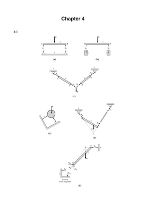
1. Chapter 4
4-1
1
RC
RA
RB
RD
C
A B
W
D
1
3 2
RB
RA
W
RB
RC
RA
2
1
W
RA
RBx
RB
RBx RBy
RBy
2
1
1
Scale of
corner magnified
W
A
B
(e)
(f)
(d)
W
A
RA RB
B
1
2
W
2
A
RA RB
B
1 1
(a) (b)
(c)

2. Chapter 4 51
4-2
(a) RA = 2 sin 60 = 1.732 kN Ans.
RB = 2 sin 30 = 1 kN Ans.
RB
(b) S = 0.6 m
α = tan−1 0.6
0.4 + 0.6
= 30.96◦
RA
sin 135
= 800
sin 30.96
⇒ RA = 1100 N Ans.
RO
sin 14.04
= 800
sin 30.96
⇒ RO = 377 N Ans.
(c)
RO = 1.2
tan 30
= 2.078 kN Ans.
RA = 1.2
sin 30
= 2.4 kN Ans.
800 N
30°
RO RA
135°
30.96°
(d) Step 1: Find RA and RE
h = 4.5
tan 30
= 7.794m
+
MA = 0
9RE − 7.794(400 cos 30) − 4.5(400 sin 30) = 0
RE = 400 N Ans.
2 4
4.5 m
Fx = 0 RAx + 400 cos 30 = 0 ⇒ RAx = −346.4N
Fy = 0 RAy + 400 − 400 sin 30 = 0 ⇒ RAy = −200N
RA =
346.42 + 2002 = 400N Ans.
D
C
h
B
y
A E x
9 m
400 N
3
30°
60°
RAy
RAx
RA
RE
1.2 kN
60°
RA
RO
90° 60°
1.2 kN
45 30.96 14.04
30.96°
RA
RO
O
0.4 m
45°
800 N
0.6 m
A
s
RA
RO
B
60°
90°
30°
2 kN
RA
2
1
2 kN
30° 60°
RA
RB

3. 52 Solutions Manual • Instructor’s Solution Manual to Accompany Mechanical Engineering Design
Step 2: Find components of RC on link 4 and RD
+
MC = 0
400(4.5) − (7.794 − 1.9)RD = 0 ⇒ RD = 305.4N Ans.
Fx = 0 ⇒ (RCx)4 = 305.4N
Fy = 0 ⇒ (RCy)4 = −400N
Step 3: Find components of RC on link 2
Fx = 0
(RCx)2 + 305.4 − 346.4 = 0 ⇒ (RCx)2 = 41N
Fy = 0
(RCy)2 = 200N
4-3
(a)
+
M0 = 0
−18(60) + 14R2 + 8(30) − 4(40) = 0
R2 = 71.43 lbf
Fy = 0: R1 − 40 + 30 + 71.43 − 60 = 0
R1 = −1.43 lbf
M1 = −1.43(4) = −5.72 lbf · in
M2 = −5.72 − 41.43(4) = −171.44 lbf · in
M3 = −171.44 − 11.43(6) = −240 lbf · in
M4 = −240 + 60(4) = 0 checks!
200 N 400 N
305.4 N
40 lbf 60 lbf
4 4 6 4
V (lbf)
1.43
41.43
60
30 lbf
11.43
x
x
x
O
A B C D
y
R1 R2
M1
M2 M3
M4
O
M
(lbf • in)
O
C C
B D
A
B D
E
305.4 N
346.4 N
305.4 N
41 N
400 N
200 N
400 N
200 N
400 N
Pin C
30°
400 N
41 N
305.4 N
200 N
346.4 N
305.4 N
(RCx)2
(RCy)2
C
B
A
2
400 N
4
RD
(RCx)4
(RCy)4
D
C
E
Ans.

4. Chapter 4 53
(b)
Fy = 0
R0 = 2 + 4(0.150) = 2.6kN
M0 = 0
M0 = 2000(0.2) + 4000(0.150)(0.425)
= 655 N · m
M1 = −655 + 2600(0.2) = −135 N · m
M2 = −135 + 600(0.150) = −45 N · m
M3 = −45 + 1
2
600(0.150) = 0 checks!
(c)
B C
M0 = 0: 10R2 − 6(1000) = 0 ⇒ R2 = 600 lbf
Fy = 0: R1 − 1000 + 600 = 0 ⇒ R1 = 400 lbf
M1 = 400(6) = 2400 lbf · ft
M2 = 2400 − 600(4) = 0 checks!
O
M
(N•m)
y 1000 lbf
R1 R2
(d) +
MC = 0
−10R1 + 2(2000) + 8(1000) = 0
R1 = 1200 lbf
Fy = 0: 1200 − 1000 − 2000 + R2 = 0
R2 = 1800 lbf
M1 = 1200(2) = 2400 lbf · ft
M2 = 2400 + 200(6) = 3600 lbf · ft
M3 = 3600 − 1800(2) = 0 checks!
1000 lbf 2000 lbf
R1
O
1200
O
M1
M2
R2
M3
2 ft 6 ft 2 ft
A B C
y
M
1800
200
x
x
x
6 ft 4 ft
A
O
O
O
B
600
M1
M2
V (lbf)
400
M
(lbf •ft)
x
x
x
V (kN)
200 mm 150 mm 150 mm
2.6
655
0.6
M1
M2
M3
y 2 kN 4 kN/m
A
O
O
O
RO MO
x
x
x

5. 54 Solutions Manual • Instructor’s Solution Manual to Accompany Mechanical Engineering Design
(e) +
MB = 0
−7R1 + 3(400) − 3(800) = 0
R1 = −171.4 lbf
Fy = 0: −171.4 − 400 + R2 − 800 = 0
R2 = 1371.4 lbf
M1 = −171.4(4) = −685.7 lbf · ft
M2 = −685.7 − 571.4(3) = −2400 lbf · ft
M3 = −2400 + 800(3) = 0 checks!
V (lbf )
400 lbf 800 lbf
4 ft 3 ft 3 ft
(f) Break at A
R1 = VA = 1
2
40(8) = 160 lbf
+
MD = 0
12(160) − 10R2 + 320(5) = 0
R2 = 352 lbf
Fy = 0
−160 + 352 − 320 + R3 = 0
R3 = 128 lbf
M1 = 1
2
160(4) = 320 lbf · in
M2 = 320 − 1
2
160(4) = 0 checks! (hinge)
M3 = 0 − 160(2) = −320 lbf · in
M4 = −320 + 192(5) = 640 lbf · in
M5 = 640 − 128(5) = 0 checks!
A
R1 VA
40 lbf/in
O
V (lbf)
160
O
O
160
320 lbf
128
A
192
M
320 lbf
160 lbf 352 lbf 128 lbf
M1
M2
M3
M4
M5
x
x
x
8
5
2
5
40 lbf/in
160 lbf
A
y
B D
C
R2 R3
O
O
O
C
M
800
171.4
571.4
B
y
M1
M2
M3
R1 R2
x
x
x

6. Chapter 4 55
4-4
(a) q = R1x−1 − 40x − 4−1 + 30x − 8−1 + R2x − 14−1 − 60x − 18−1
V = R1 − 40x − 40 + 30x − 80 + R2x − 140 − 60x − 180 (1)
M = R1x − 40x − 41 + 30x − 81 + R2x − 141 − 60x − 181 (2)
for x = 18+ V = 0 and M = 0 Eqs. (1) and (2) give
0 = R1 − 40 + 30 + R2 − 60 ⇒ R1 + R2 = 70 (3)
0 = R1(18) − 40(14) + 30(10) + 4R2 ⇒ 9R1 + 2R2 = 130 (4)
Solve (3) and (4) simultaneously to get R1 = −1.43 lbf, R2 = 71.43 lbf. Ans.
From Eqs. (1) and (2), at x = 0+, V = R1 = −1.43 lbf, M = 0
x = 4+: V = −1.43 − 40 = −41.43, M = −1.43x
x = 8+: V = −1.43 − 40 + 30 = −11.43
M = −1.43(8) − 40(8 − 4)1 = −171.44
x = 14+: V = −1.43 − 40 + 30 + 71.43 = 60
M = −1.43(14) − 40(14 − 4) + 30(14 − 8) = −240.
x = 18+: V = 0, M = 0 See curves of V and M in Prob. 4-3 solution.
(b) q = R0x−1 − M0x−2 − 2000x − 0.2−1 − 4000x − 0.350 + 4000x − 0.50
V = R0 − M0x−1 − 2000x − 0.20 − 4000x − 0.351 + 4000x − 0.51 (1)
M = R0x − M0 − 2000x − 0.21 − 2000x − 0.352 + 2000x − 0.52 (2)
at x = 0.5+m, V = M = 0, Eqs. (1) and (2) give
R0 − 2000 − 4000(0.5 − 0.35) = 0 ⇒ R1 = 2600N = 2.6 kN Ans.
R0(0.5) − M0 − 2000(0.5 − 0.2) − 2000(0.5 − 0.35)2 = 0
with R0 = 2600 N, M0 = 655 N · m Ans.
With R0 and M0, Eqs. (1) and (2) give the same V and M curves as Prob. 4-3 (note for
V, M0x−1 has no physical meaning).
(c) q = R1x−1 − 1000x − 6−1 + R2x − 10−1
V = R1 − 1000x − 60 + R2x − 100 (1)
M = R1x − 1000x − 61 + R2x − 101 (2)
at x = 10+ ft, V = M = 0, Eqs. (1) and (2) give
R1 − 1000 + R2 = 0 ⇒ R1 + R2 = 1000
10R1 − 1000(10 − 6) = 0 ⇒ R1 = 400 lbf , R2 = 1000 − 400 = 600 lbf
0 ≤ x ≤ 6: V = 400 lbf, M = 400x
6 ≤ x ≤ 10: V = 400 − 1000(x − 6)0 = 600 lbf
M = 400x − 1000(x − 6) = 6000 − 600x
See curves of Prob. 4-3 solution.

7. 56 Solutions Manual • Instructor’s Solution Manual to Accompany Mechanical Engineering Design
(d) q = R1x−1 − 1000x − 2−1 − 2000x − 8−1 + R2x − 10−1
V = R1 − 1000x − 20 − 2000x − 80 + R2x − 100 (1)
M = R1x − 1000x − 21 − 2000x − 81 + R2x − 101 (2)
At x = 10+, V = M = 0 from Eqs. (1) and (2)
R1 − 1000 − 2000 + R2 = 0 ⇒ R1 + R2 = 3000
10R1 − 1000(10 − 2) − 2000(10 − 8) = 0 ⇒ R1 = 1200 lbf ,
R2 = 3000 − 1200 = 1800 lbf
0 ≤ x ≤ 2: V = 1200 lbf, M = 1200x lbf · ft
2 ≤ x ≤ 8: V = 1200 − 1000 = 200 lbf
M = 1200x − 1000(x − 2) = 200x + 2000 lbf · ft
8 ≤ x ≤ 10: V = 1200 − 1000 − 2000 = −1800 lbf
M = 1200x − 1000(x − 2) − 2000(x − 8) = −1800x + 18 000 lbf · ft
Plots are the same as in Prob. 4-3.
(e) q = R1x−1 − 400x − 4−1 + R2x − 7−1 − 800x − 10−1
V = R1 − 400x − 40 + R2x − 70 − 800x − 100 (1)
M = R1x − 400x − 41 + R2x − 71 − 800x − 101 (2)
at x = 10+, V = M = 0
R1 − 400 + R2 − 800 = 0 ⇒ R1 + R2 = 1200 (3)
10R1 − 400(6) + R2(3) = 0 ⇒ 10R1 + 3R2 = 2400 (4)
Solve Eqs. (3) and (4) simultaneously: R1 = −171.4 lbf, R2 = 1371.4 lbf
0 ≤ x ≤ 4: V = −171.4 lbf, M = −171.4x lbf · ft
4 ≤ x ≤ 7: V = −171.4 − 400 = −571.4 lbf
M=−171.4x − 400(x − 4) lbf · ft =−571.4x + 1600
7 ≤ x ≤ 10: V = −171.4 − 400 + 1371.4 = 800 lbf
M=−171.4x − 400(x − 4) + 1371.4(x − 7) = 800x − 8000 lbf · ft
Plots are the same as in Prob. 4-3.
(f ) q = R1x−1 − 40x0 + 40x − 80 + R2x − 10−1 − 320x − 15−1 + R3x − 20
V = R1 − 40x + 40x − 81 + R2x − 100 − 320x − 150 + R3x − 200 (1)
M = R1x − 20x2 + 20x − 82 + R2x − 101 − 320x − 151 + R3x − 201 (2)
M = 0 at x = 8 in ∴8R1 − 20(8)2 = 0 ⇒ R1 = 160 lbf
at x = 20+, V and M = 0
160 − 40(20) + 40(12) + R2 − 320 + R3 = 0 ⇒ R2 + R3 = 480
160(20) − 20(20)2 + 20(12)2 + 10R2 − 320(5) = 0 ⇒ R2 = 352 lbf
R3 = 480 − 352 = 128 lbf
0 ≤ x ≤ 8: V = 160 − 40x lbf, M = 160x − 20x2 lbf · in
8 ≤ x ≤ 10: V = 160 − 40x + 40(x − 8) = −160 lbf ,
M = 160x − 20x2 + 20(x − 8)2 = 1280 − 160x lbf · in

8. Chapter 4 57
10 ≤ x ≤ 15: V = 160 − 40x + 40(x − 8) + 352 = 192 lbf
M = 160x − 20x2 + 20(x − 8) + 352(x − 10) = 192x − 2240
15 ≤ x ≤ 20: V = 160 − 40x + 40(x − 8) + 352 − 320 = −128 lbf
M = 160x − 20x2 − 20(x − 8) + 352(x − 10) − 320(x − 15)
=−128x + 2560
Plots of V and M are the same as in Prob. 4-3.
4-5 Solution depends upon the beam selected.
4-6
(a) Moment at center, xc = (l − 2a)/2
Mc = w
2
l
2
(l − 2a) −
l
2
2
= wl
2
l
4
− a
At reaction, |Mr| = wa2/2
a = 2.25, l = 10 in, w = 100 lbf/in
Mc = 100(10)
2
10
4
= 125 lbf · in
− 2.25
Mr = 100(2.252)
2
= 253.1 lbf · in Ans.
(b) Minimum occurs when Mc = |Mr |
wl
2
l
4
− a
= wa2
2
⇒ a2 + al − 0.25l2 = 0
Taking the positive root
a = 1
2
−l +
l2 + 4(0.25l2)
= l
2
√
= 0.2071l Ans.
2 − 1
for l = 10 in and w = 100 lbf, Mmin = (100/2)[(0.2071)(10)]2 = 214.5 lbf · in
4-7 For the ith wire from bottom, from summing forces vertically
(a)
Ti = (i + 1)W
Ti
xi
a
From summing moments about point a,
Ma = W(l − xi ) − iWxi = 0
Giving,
xi = l
i + 1
W iW

9. 58 Solutions Manual • Instructor’s Solution Manual to Accompany Mechanical Engineering Design
So
W = l
1 + 1
= l
2
x = l
2 + 1
= l
3
y = l
3 + 1
= l
4
z = l
4 + 1
= l
5
(b) With straight rigid wires, the mobile is not stable. Any perturbation can lead to all wires
becoming collinear. Consider a wire of length l bent at its string support:
Ma = 0
Ma = iWl
i + 1
cos α − ilW
i + 1
cos β = 0
iWl
i + 1
(cos α − cos β) = 0
W iW
Moment vanishes when α = β for any wire. Consider a ccw rotation angle β, which
makes α →α + β and β →α − β
Ma = iWl
i + 1
[cos(α + β) − cos(α − β)]
= 2iWl
i + 1
sin α sin β
.=
2iWlβ
i + 1
sin α
There exists a correcting moment of opposite sense to arbitrary rotation β. An equation
for an upward bend can be found by changing the sign of W. The moment will no longer
be correcting. A curved, convex-upward bend of wire will produce stable equilibrium
too, but the equation would change somewhat.
4-8
(a)
C = 12 + 6
2
= 9
CD = 12 − 6
2
= 3
R =
32 + 42 = 5
σ1 = 5 + 9 = 14
σ2 = 9 − 5 = 4
2s
(12, 4cw)
1
C
R
D
2
1
2
2p
(6, 4ccw)
y
x
cw
ccw
il
i 1
Ti
l
i 1

10. Chapter 4 59
φp = 1
2
tan−1
4
3
= 26.6◦ cw
τ1 = R = 5, φs = 45◦ − 26.6◦ = 18.4◦ ccw
(b)
C = 9 + 16
2
= 12.5
CD = 16 − 9
2
= 3.5
R =
52 + 3.52 = 6.10
σ1 = 6.1 + 12.5 = 18.6
φp = 1
2
tan−1 5
3.5
= 27.5◦ ccw
σ2 = 12.5 − 6.1 = 6.4
y
2 1
x
1
τ1 = R = 6.10, φs = 45◦ − 27.5◦ = 17.5◦ cw
(c)
C = 24 + 10
2
= 17
CD = 24 − 10
2
= 7
R =
72 + 62 = 9.22
σ1 = 17 + 9.22 = 26.22
σ2 = 17 − 9.22 = 7.78
6.10
2 1
2s
(24, 6cw)
C
R
D
1
2
2p
(10, 6ccw)
y
x
cw
ccw
x
12.5
12.5
17.5
6.4
18.6
27.5
2s
(16, 5ccw)
C
R
D
2
2p
(9, 5cw)
x
cw
ccw
3
5
3
3
3
18.4
x
x
4
14
26.6

11. 60 Solutions Manual • Instructor’s Solution Manual to Accompany Mechanical Engineering Design
φp = 1
2
90 + tan−1 7
6

12. = 69.7◦ ccw
x
τ1 = R = 9.22, φs = 69.7◦ − 45◦ = 24.7◦ ccw
(d)
C = 9 + 19
2
= 14
CD = 19 − 9
2
= 5
R =
52 + 82 = 9.434
σ1 = 14 + 9.43 = 23.43
σ2 = 14 − 9.43 = 4.57
2 1
φp = 1
2
90 + tan−1 5
8

13. = 61.0◦ cw
2s
1
τ1 = R = 9.434, φs = 61◦ − 45◦ = 16◦ cw
x
14
14
9.434
16
x
23.43
4.57
61
(9, 8cw)
C
R
D
2
2p
(19, 8ccw)
y
x
cw
ccw
x
17
17
9.22
24.7
26.22
7.78
69.7

14. Chapter 4 61
4-9
(a)
C = 12 − 4
2
= 4
CD = 12 + 4
2
= 8
R =
82 + 72 = 10.63
σ1 = 4 + 10.63 = 14.63
σ2 = 4 − 10.63 = −6.63
φp = 1
2
90 + tan−1 8
7

15. = 69.4◦ ccw
x
1
τ1 = R = 10.63, φs = 69.4◦ − 45◦ = 24.4◦ ccw
(b)
C = 6 − 5
2
= 0.5
CD = 6 + 5
2
= 5.5
R =
5.52 + 82 = 9.71
σ1 = 0.5 + 9.71 = 10.21
σ2 = 0.5 − 9.71 = −9.21
φp = 1
2
tan−1 8
5.5
= 27.75◦ ccw
x
10.21
9.21
2s
27.75
(5, 8cw)
1
C
R
D
2
1
2
2p
(6, 8ccw)
y
x
cw
ccw
x
4
4
10.63
24.4
14.63
6.63
69.4
2s
(12, 7cw)
C
R
D
2
1
2
2p
(4, 7ccw)
y
x
cw
ccw

16. 62 Solutions Manual • Instructor’s Solution Manual to Accompany Mechanical Engineering Design
τ1 = R = 9.71, φs = 45◦ − 27.75◦ = 17.25◦ cw
(c)
C =
−8 + 7
2
= −0.5
CD = 8 + 7
2
= 7.5
R =
7.52 + 62 = 9.60
σ1 = 9.60 − 0.5 = 9.10
σ2 = −0.5 − 9.6 = −10.1
9.71
2 1
φp = 1
2
90 + tan−1 7.5
6

17. = 70.67◦ cw
x
1
τ1 = R = 9.60, φs = 70.67◦ − 45◦ = 25.67◦ cw
(d)
C = 9 − 6
2
= 1.5
CD = 9 + 6
2
= 7.5
R =
7.52 + 32 = 8.078
σ1 = 1.5 + 8.078 = 9.58
σ2 = 1.5 − 8.078 = −6.58
2s
(9, 3cw)
1
2 1
R C D
2
2p
(6, 3ccw)
y
x
cw
ccw
x
0.5
0.5
9.60
25.67
10.1
9.1
70.67
2s
(8, 6cw)
C
R
D
2
2p
(7, 6ccw)
x
y
cw
ccw
x
0.5
0.5
17.25

18. Chapter 4 63
φp = 1
2
tan−1 3
7.5
= 10.9◦ cw
τ1 = R = 8.078, φs = 45◦ − 10.9◦ = 34.1◦ ccw
4-10
(a)
C = 20 − 10
2
= 5
CD = 20 + 10
2
= 15
R =
152 + 82 = 17
σ1 = 5 + 17 = 22
σ2 = 5 − 17 = −12
2s (20, 8cw)
2 1
φp = 1
2
tan−1 8
15
= 14.04◦ cw
1
τ1 = R = 17, φs = 45◦ − 14.04◦ = 30.96◦ ccw
5
17
5
30.96
x
12
22
14.04
x
C
R
D
2
2p
(10, 8ccw)
y
x
cw
ccw
x
1.5
8.08
1.5
34.1
x
6.58
9.58
10.9

19. 64 Solutions Manual • Instructor’s Solution Manual to Accompany Mechanical Engineering Design
(b)
C = 30 − 10
2
= 10
CD = 30 + 10
2
= 20
R =
202 + 102 = 22.36
σ1 = 10 + 22.36 = 32.36
σ2 = 10 − 22.36 = −12.36
φp = 1
2
tan−1 10
20
= 13.28◦ ccw
2s
1
τ1 = R = 22.36, φs = 45◦ − 13.28◦ = 31.72◦ cw
(c)
C =
−10 + 18
2
= 4
CD = 10 + 18
2
= 14
R =
142 + 92 = 16.64
σ1 = 4 + 16.64 = 20.64
σ2 = 4 − 16.64 = −12.64
10
22.36
10
2 1
φp = 1
2
90 + tan−1 14
9

20. = 73.63◦ cw
1
τ1 = R = 16.64, φs = 73.63◦ − 45◦ = 28.63◦ cw
4
x
16.64
4
28.63
12.64
20.64
73.63
x
(10, 9cw) 2s
C
R
D
2
2p
(18, 9ccw)
y
x
cw
ccw
31.72
x
12.36
32.36
x
13.28
(10, 10cw)
C
R
D
2
1
2 2p
(30, 10ccw)
y
x
cw
ccw

21. Chapter 4 65
(d)
C =
−12 + 22
2
= 5
CD = 12 + 22
2
= 17
R =
172 + 122 = 20.81
σ1 = 5 + 20.81 = 25.81
σ2 = 5 − 20.81 = −15.81
2 1
φp = 1
2
90 + tan−1 17
12

22. = 72.39◦ cw
1
τ1 = R = 20.81, φs = 72.39◦ − 45◦ = 27.39◦ cw
4-11
(a)
(b)
C = 0 + 10
2
= 5
CD = 10 − 0
2
= 5
R =
52 + 42 = 6.40
σ1 = 5 + 6.40 = 11.40
σ2 = 0, σ3 = 5 − 6.40 = −1.40
14
2
1/3 7
4 y x 10
1/3
τ1/3 = R = 6.40, τ1/2 = 11.40
2
= 5.70, τ2/3 = 1.40
2
= 0.70
2 1
3
D
x
y
C
R
(0, 4cw)
(10, 4ccw)
2/3
1/2
x 1
3 y
2 0
2/3 2
1/2 5
5
20.81
5
27.39
x
15.81
25.81
72.39
x
(12, 12cw) 2s
C
R
D
2
2p
(22, 12ccw)
y
x
cw
ccw

23. 66 Solutions Manual • Instructor’s Solution Manual to Accompany Mechanical Engineering Design
(c)
C =
−2 − 8
2
= −5
CD = 8 − 2
2
= 3
R =
32 + 42 = 5
σ1 = −5 + 5 = 0, σ2 = 0
σ3 = −5 − 5 = −10
τ1/3 = 10
2
= 5, τ1/2 = 0, τ2/3 = 5
(d)
C = 10 − 30
2
= −10
CD = 10 + 30
2
= 20
R =
202 + 102 = 22.36
σ1 = −10 + 22.36 = 12.36
σ2 = 0
σ3 = −10 − 22.36 = −32.36
2/3
τ1/3 = 22.36, τ1/2 = 12.36
2
1
= 6.18, τ2/3 = 32.36
2
= 16.18
4-12
(a)
C =
−80 − 30
2
= −55
CD = 80 − 30
2
= 25
R =
252 + 202 = 32.02
σ1 = 0
σ2 = −55 + 32.02 = −22.98 = −23.0
σ3 = −55 − 32.0 = −87.0
x
τ1/2 = 23
2
C
= 11.5, τ2/3 = 32.0, τ1/3 = 87
2
= 43.5
1
(80, 20cw)
(30, 20ccw)
D
R
2/3
1/2
1/3
3 2
y
(30, 10cw)
(10, 10ccw)
C D
R
1/2
1/3
3 2
y
x
12
3
(2, 4cw)
Point is a circle
2 circles
C
D
y
x
(8, 4ccw)

24. Chapter 4 67
(b)
C = 30 − 60
2
= −15
CD = 60 + 30
2
= 45
R =
452 + 302 = 54.1
σ1 = −15 + 54.1 = 39.1
σ2 = 0
σ3 = −15 − 54.1 = −69.1
τ1/3 = 39.1 + 69.1
2
R
= 54.1, τ1/2 = 39.1
2
= 19.6, τ2/3 = 69.1
2
= 34.6
(c)
C = 40 + 0
2
= 20
CD = 40 − 0
2
= 20
R =
202 + 202 = 28.3
σ1 = 20 + 28.3 = 48.3
σ2 = 20 − 28.3 = −8.3
σ3 = σz = −30
C
y
τ1/3 = 48.3 + 30
2
= 39.1, τ1/2 = 28.3, τ2/3 = 30 − 8.3
2
= 10.9
(d)
C = 50
2
= 25
CD = 50
2
= 25
R =
252 + 302 = 39.1
σ1 = 25 + 39.1 = 64.1
σ2 = 25 − 39.1 = −14.1
σ3 = σz = −20
1/3
C D
τ1/3 = 64.1 + 20
2
(50, 30cw)
= 42.1, τ1/2 = 39.1, τ2/3 = 20 − 14.1
2
= 2.95
1
(0, 30ccw)
2/3
1/2
3 2
x
y
1
(0, 20cw)
(40, 20ccw)
D
R
2/3
1/2
1/3
3 2
x
1
(60, 30ccw)
(30, 30cw)
C D
2/3
1/2
1/3
3 2
x
y

25. 68 Solutions Manual • Instructor’s Solution Manual to Accompany Mechanical Engineering Design
4-13
σ = F
A
= 2000
(π/4)(0.52)
= 10 190 psi = 10.19 kpsi Ans.
δ = FL
AE
= σ
L
E
= 10 190
72
30(106)
= 0.024 46 in Ans.
1 = δ
L
= 0.024 46
72
= 340(10−6) = 340μ Ans.
From Table A-5, ν = 0.292
2 = −ν1 = −0.292(340) = −99.3μ Ans.
d = 2d = −99.3(10−6)(0.5) = −49.6(10−6) in Ans.
4-14 From Table A-5, E = 71.7 GPa
δ = σ
L
E
= 135(106)
3
71.7(109)
= 5.65(10−3) m = 5.65 mm Ans.
4-15 From Table 4-2, biaxial case. From Table A-5, E = 207 GPa and ν = 0.292
σx = E(x + νy)
1 − ν2
= 207(109)[0.0021 + 0.292(−0.000 67)]
1 − 0.2922 (10−6) = 431MPa Ans.
σy = 207(109)[−0.000 67 + 0.292(0.0021)]
1 − 0.2922 (10−6) = −12.9MPa Ans.
4-16 The engineer has assumed the stress to be uniform. That is,
Ft = −F cos θ + τ A = 0 ⇒ τ = F
A
cos θ
When failure occurs in shear
Ssu = F
A
cos θ
The uniform stress assumption is common practice but is not exact. If interested in the
details, see p. 570 of 6th edition.
4-17 From Eq. (4-15)
σ3 − (−2 + 6 − 4)σ2 + [−2(6) + (−2)(−4) + 6(−4) − 32 − 22 − (−5)2]σ
−[−2(6)(−4) + 2(3)(2)(−5) − (−2)(2)2 − 6(−5)2 − (−4)(3)2] = 0
σ3 − 66σ + 118 = 0
Roots are: 7.012, 1.89, −8.903 kpsi Ans.
t
F

26. Chapter 4 69
τ1/2 = 7.012 − 1.89
2
= 2.56 kpsi
τ2/3 = 8.903 + 1.89
2
= 5.40 kpsi
τmax = τ1/3 = 8.903 + 7.012
2
= 7.96 kpsi Ans.
Note: For Probs. 4-17 to 4-19, one can also find the eigenvalues of the matrix
[σ] =
σx τxy τzx
τxy σy τyz
τzx τyz σz
for the principal stresses
4-18 From Eq. (4-15)
σ3 − (10 + 0 + 10)σ2 +
10(0) + 10(10) + 0(10) − 202 −
√
2
−10
2 − 02
σ
−
10(0)(10) + 2(20)
√
2
−10
(0) − 10
√
2
−10
2 − 0(0)2 − 10(20)2
= 0
σ3 − 20σ2 − 500σ + 6000 = 0
Roots are: 30, 10, −20 MPa Ans.
τ1/2 = 30 − 10
2
= 10MPa
τ2/3 = 10 + 20
2
= 15MPa
τmax = τ1/3 = 30 + 20
2
= 25 MPa Ans.
4-19 From Eq. (4-15)
2/3
1/2
1/3
σ3 − (1 + 4 + 4)σ2 + [1(4) + 1(4) + 4(4) − 22 − (−4)2 − (−2)2]σ
−[1(4)(4) + 2(2)(−4)(−2) − 1(−4)2 − 4(−2)2 − 4(2)2] = 0
σ3 − 9σ2 = 0
20 10 30
(MPa)
(MPa)
1.89 7.012
8.903
2/3
1/2
1/3
(kpsi)
(kpsi)

27. 70 Solutions Manual • Instructor’s Solution Manual to Accompany Mechanical Engineering Design
Roots are: 9, 0, 0 kpsi
(kpsi)
τ2/3 = 0, τ1/2 = τ1/3 = τmax = 9
2
= 4.5 kpsi Ans.
4-20
(a) R1 = c
l
F Mmax = R1a = ac
l
F
σ = 6M
bh2
= 6
bh2
ac
l
F ⇒ F = σbh2l
6ac
Ans.
(b)
Fm
F
= (σm/σ )(bm/b) (hm/h)2 (lm/l)
(am/a) (cm/c)
= 1(s)(s)2(s)
(s)(s)
= s2 Ans.
For equal stress, the model load varies by the square of the scale factor.
4-21
R1 = wl
2
, Mmax|x=l/2 = w
2
l
2
l − l
2
= wl2
8
σ = 6M
bh2
= 6
bh2
wl2
8
= 3Wl
4bh2
⇒ W = 4
3
σbh2
l
Ans.
Wm
W
= (σm/σ)(bm/b) (hm/h)2
lm/l
= 1(s)(s)2
s
= s2 Ans.
wmlm
wl
= s2 ⇒ wm
w
= s2
s
= s Ans.
For equal stress, the model load w varies linearily with the scale factor.
4-22
(a) Can solve by iteration or derive equations for the general case.
Find maximum moment under wheel W3
WT = W at centroid of W’s
RA = l − x3 − d3
l
WT
RA
W1
W2 W3 . . . WT . . .
A B
d3
Wn
RB
a23
a13
x3
l
2/3
(kpsi)
1/2 1/3
O0 9

28. Chapter 4 71
Under wheel 3
M3 = RAx3 − W1a13 − W2a23 = (l − x3 − d3)
l
WT x3 − W1a13 − W2a23
For maximum,
dM3
dx3
= 0 = (l − d3 − 2x3)
WT
l
⇒ x3 = l − d3
2
substitute into M, ⇒ M3 = (l − d3)2
4l
WT − W1a13 − W2a23
This means the midpoint of d3 intersects the midpoint of the beam
For wheel i xi = l − di
2
, Mi = (l − di )2
4l
WT −
i−1
j=1
Wjaji
Note for wheel 1:

29. Wjaji = 0
WT = 104.4, W1 = W2 = W3 = W4 = 104.4
4
= 26.1 kip
Wheel 1: d1 = 476
2
= 238 in, M1 = (1200 − 238)2
4(1200)
(104.4) = 20 128 kip · in
Wheel 2: d2 = 238 − 84 = 154 in
M2 = (1200 − 154)2
4(1200)
(104.4) − 26.1(84) = 21 605 kip · in = Mmax
Check if all of the wheels are on the rail
(b) xmax = 600 − 77 = 523 in
(c) See above sketch.
(d) inner axles
4-23
(a)
84 77 84
315
xmax
a a
C
Ga
c1 0.833
0.75
1 1
Gb
b
1 1
1
2 4
3
8
1
4
1
4
D
0.167
Aa = Ab = 0.25(1.5) = 0.375 in2
A = 3(0.375) = 1.125 in2
0.083
0.5
1.5
y c2 0.667
B
A
600 600

30. 72 Solutions Manual • Instructor’s Solution Manual to Accompany Mechanical Engineering Design
¯y = 2(0.375)(0.75) + 0.375(0.5)
1.125
= 0.667 in
Ia = 0.25(1.5)3
12
= 0.0703 in4
Ib = 1.5(0.25)3
12
= 0.001 95 in4
I1 = 2[0.0703 + 0.375(0.083)2] + [0.001 95 + 0.375(0.167)2] = 0.158 in4 Ans.
σA = 10 000(0.667)
0.158
= 42(10)3 psi Ans.
σB = 10 000(0.667 − 0.375)
0.158
= 18.5(10)3 psi Ans.
σC = 10 000(0.167 − 0.125)
0.158
= 2.7(10)3 psi Ans.
σD = −10 000(0.833)
0.158
= −52.7(10)3 psi Ans.
(b)
D
C
1 1
B
A
y
Here we treat the hole as a negative area.
Aa = 1.732 in2
Ab = 1.134
0.982
2
= 0.557 in2
A = 1.732 − 0.557 = 1.175 in2
¯y = 1.732(0.577) − 0.557(0.577)
1.175
a b
Ga 0.327 Gb
= 0.577 in Ans.
Ia = bh3
36
= 2(1.732)3
36
= 0.289 in4
Ib = 1.134(0.982)3
36
= 0.0298 in4
I1 = Ia − Ib = 0.289 − 0.0298 = 0.259 in4 Ans.
A
0.25
c1 1.155
c2 0.577
2
1.732
0.577
0.982
0.577
1.134

31. Chapter 4 73
because the centroids are coincident.
σA = 10 000(0.577)
0.259
= 22.3(10)3 psi Ans.
σB = 10 000(0.327)
0.259
= 12.6(10)3 psi Ans.
σC = −10 000(0.982 − 0.327)
0.259
= −25.3(10)3 psi Ans.
σD = −10 000(1.155)
0.259
= −44.6(10)3 psi Ans.
(c) Use two negative areas.
D
C
1 1
B
Gb Gc
Aa = 1 in2, Ab = 9 in2, Ac = 16 in2, A = 16 − 9 − 1 = 6 in2;
¯ya = 0.25 in, ¯yb = 2.0 in, ¯yc = 2 in
¯y = 16(2) − 9(2) − 1(0.25)
6
= 2.292 in Ans.
c1 = 4 − 2.292 = 1.708 in
Ia = 2(0.5)3
12
= 0.020 83 in4
Ib = 3(3)3
12
= 6.75 in4
Ic = 4(4)3
12
= 21.333 in4
I1 = [21.333 + 16(0.292)2] − [6.75 + 9(0.292)2]
−[0.020 83 + 1(2.292 − 0.25)2]
= 10.99 in4 Ans.
σA = 10 000(2.292)
10.99
= 2086 psi Ans.
σB = 10 000(2.292 − 0.5)
10.99
= 1631 psi Ans.
σC = −10 000(1.708 − 0.5)
10.99
= −1099 psi Ans.
σD = −10 000(1.708)
10.99
= −1554 psi Ans.
c
a
b
A
Ga
c1 1.708
c2 2.292
2
1.5
0.25

32. 74 Solutions Manual • Instructor’s Solution Manual to Accompany Mechanical Engineering Design
(d) Use a as a negative area.
B
1 1
Aa = 6.928 in2, Ab = 16 in2, A = 9.072 in2;
¯ya = 1.155 in, ¯yb = 2 in
¯y = 2(16) − 1.155(6.928)
9.072
= 2.645 in Ans.
c1 = 4 − 2.645 = 1.355 in
Ia = bh3
36
= 4(3.464)3
36
= 4.618 in4
Ib = 4(4)3
12
= 21.33 in4
I1 = [21.33 + 16(0.645)2] − [4.618 + 6.928(1.490)2]
= 7.99 in4 Ans.
σA = 10 000(2.645)
7.99
= 3310 psi Ans.
σB = −10 000(3.464 − 2.645)
7.99
= −1025 psi Ans.
σC = −10 000(1.355)
7.99
= −1696 psi Ans.
(e) Aa = 6(1.25) = 7.5 in2
Ab = 3(1.5) = 4.5 in2
A = Ac + Ab = 12 in2
¯y = 3.625(7.5) + 1.5(4.5)
12
= 2.828 in Ans.
I = 1
12
C
(6)(1.25)3 + 7.5(3.625 − 2.828)2 + 1
12
(1.5)(3)3 + 4.5(2.828 − 1.5)2
= 17.05 in4 Ans.
σA = 10 000(2.828)
17.05
= 1659 psi Ans.
σB = −10 000(3 − 2.828)
17.05
= −101 psi Ans.
σC = −10 000(1.422)
17.05
= −834 psi Ans.
a
b
A
B
c1 1.422
c2 2.828
3.464
Ga
b
a
C
A
c1 1.355
c2 2.645
1.490
1.155

33. Chapter 4 75
(f) Let a = total area
A = 1.5(3) − 1(1.25) = 3.25 in2
I = Ia − 2Ib = 1
12
(1.5)(3)3 − 1
12
(1.25)(1)3
= 3.271 in4 Ans.
σA = 10 000(1.5)
3.271
= 4586 psi, σD = −4586 psi
Ans.
σB = 10 000(0.5)
3.271
= 1529 psi, σC = −1529 psi
4-24
(a) The moment is maximum and constant between A and B
M = −50(20) = −1000 lbf · in , I = 1
12
(0.5)(2)3 = 0.3333 in4
ρ =
E I
M
= 1.6(106)(0.3333)
1000
= 533.3 in
(x, y) = (30, −533.3) in Ans.
(b) The moment is maximum and constant between A and B
M = 50(5) = 250 lbf · in, I = 0.3333 in4
ρ = 1.6(106)(0.3333)
250
= 2133 in Ans.
(x, y) = (20, 2133) in Ans.
4-25
(a)
I = 1
12
(0.75)(1.5)3 = 0.2109 in4
A = 0.75(1.5) = 1.125 in
Mmax is at A. At the bottom of the section,
σmax = Mc
I
= 4000(0.75)
0.2109
= 14 225 psi Ans.
Due to V, τmax constant is between A and B
at y = 0
τmax = 3
2
V
A
= 3
2
667
1.125
= 889 psi Ans.
1000 lbf
O B
333 lbf 667 lbf
4000
x
A
333
O
667
O
12 6
V (lbf)
M
(lbf •in)
x
C
B
A
b
a
b
D
c 1.5
c 1.5
1.5

34. 76 Solutions Manual • Instructor’s Solution Manual to Accompany Mechanical Engineering Design
(b)
I = 1
12
(1)(2)3 = 0.6667 in4
Mmax is at A at the top of the beam
σmax = 8000(1)
0.6667
= 12 000 psi Ans.
|Vmax| = 1000 lbf from O to B at y = 0
τmax = 3
2
V
A
= 3
2
1000
(2)(1)
= 750 psi Ans.
(c)
I = 1
12
(0.75)(2)3 = 0.5 in4
M1 = −1
2
600(5) = −1500 lbf · in = M3
M2 = −1500 + 1
2
(900)(7.5) = 1875 lbf · in
Mmax is at span center. At the bottom of the
beam,
σmax = 1875(1)
0.5
= 3750 psi Ans.
At A and B at y = 0
τmax = 3
2
900
(0.75)(2)
= 900 psi Ans.
(d)
I = 1
12
(1)(2)3 = 0.6667 in4
M1 = −600
2
(6) = −1800 lbf · in
M2 = −1800 + 1
2
750(7.5) = 1013 lbf · in
At A, top of beam
σmax = 1800(1)
0.6667
= 2700 psi Ans.
At A, y = 0
τmax = 3
2
750
(2)(1)
= 563 psi Ans.
O B
100 lbf/in
V (lbf)
M
(lbf •in)
900
O A B
1350 lbf 450 lbf
V (lbf)
O
M
(lbf •in)
O
6 12
7.5
750
M1
450
M2
600
x
x
x
120 lbf/in
1500 lbf 1500 lbf
O
A B C
O
O
5 15 5
900
M1
M2
x
x
M3
600
600
x
x
1000 lbf 1000 lbf
1000
1000
8000
2000 lbf
A
O
O
8 8
V (lbf)
M
(lbf •in)
x
x

35. Chapter 4 77
4-26
Mmax = wl2
8
⇒ σmax = wl2c
8I
⇒ w = 8σ I
cl2
(a) l = 12(12) = 144 in, I = (1/12)(1.5)(9.5)3 = 107.2 in4
w = 8(1200)(107.2)
4.75(1442)
= 10.4 lbf/in Ans.
(b) l = 48 in, I = (π/64)(24 − 1.254) = 0.6656 in4
w = 8(12)(103)(0.6656)
1(48)2
= 27.7 lbf/in Ans.
(c) l = 48 in, I .=
(1/12)(2)(33) − (1/12)(1.625)(2.6253) = 2.051 in4
w = 8(12)(103)(2.051)
1.5(48)2
= 57.0 lbf/in Ans.
(d) l = 72 in; Table A-6, I = 2(1.24) = 2.48 in4
cmax = 2.158
w = 8(12)(103)(2.48)
2.158(72)2
= 21.3 lbf/in Ans.
(e) l = 72 in; Table A-7, I = 3.85 in4
w = 8(12)(103)(3.85)
2(722)
= 35.6 lbf/in Ans.
(f) l = 72 in, I = (1/12)(1)(43) = 5.333 in4
w = 8(12)(103)(5.333)
(2)(72)2
= 49.4 lbf/in Ans.
4-27 (a) Model (c)
I = π
64
(0.54) = 3.068(10−3) in4
A = π
4
(0.52) = 0.1963 in2
σ = Mc
I
= 218.75(0.25)
3.068(10−3)
= 17 825 psi = 17.8 kpsi Ans.
τmax = 4
3
V
A
= 4
3
500
0.1963
= 3400 psi Ans.
500 lbf 500 lbf
1.25 in
0.4375
500 lbf 500 lbf
500
500
V (lbf)
O
M
(lbf ¥in)
O
Mmax 500(0.4375)
218.75 lbf ¥in
2
0.842
2.158

36. 78 Solutions Manual • Instructor’s Solution Manual to Accompany Mechanical Engineering Design
(b) Model (d)
Mmax = 500(0.25) + 1
2
(500)(0.375)
= 218.75 lbf · in
Vmax = 500 lbf
Same M and V
∴ σ = 17.8 kpsi Ans.
τmax = 3400 psi Ans.
0.25
1333 lbf/in
V (lbf)
M Mmax
4-28 If support RB is between F1 and F2 at position x = l, maximum moments occur at x = 3 and l.
MB = RAl − 2000(l − 3) + 1100(7.75 − l) = 0
RA = 3100 − 14 525/l
Mx=3 = 3RA = 9300 − 43 575/l
MB = RAl − 2000(l − 3) = 1100 l − 8525
To minimize the moments, equate Mx=3 to −MB giving
9300 − 43 575/l = −1100l + 8525
Multiply by l and simplify to
l2 + 0.7046l − 39.61 = 0
The positive solution for l is 5.95 in and the magnitude of the moment is
M = 9300 − 43 575/5.95 = 1976 lbf · in
Placing the bearing to the right of F2, the bending moment would be minimized by placing
it as close as possible to F2. If the bearing is near point B as in the original figure, then we
need to equate the reaction forces. From statics, RB = 14 525/l, and RA = 3100 − RB.
For RA = RB, then RA = RB = 1550 lbf, and l = 14 575/1550 = 9.37 in.
4-29
l p2
p1
q = −Fx−1 + p1x − l0 − p1 + p2
a
a
b
x − l1 + terms for x l + a
V = −F + p1x − l1 − p1 + p2
2a
x − l2 + terms for x l + a
M = −Fx + p1
2
x − l2 − p1 + p2
6a
x − l3 + terms for x l + a
F
1.25
500 lbf 500 lbf
500
500
O
O

37. Chapter 4 79
At x = (l + a)+, V = M = 0, terms for x l + a = 0
−F + p1a − p1 + p2
2a
a2 = 0 ⇒ p1 − p2 = 2F
a
(1)
−F(l + a) + p1a2
2
− p1 + p2
6a
a3 = 0 ⇒ 2p1 − p2 = 6F(l + a)
a2 (2)
From (1) and (2) p1 = 2F
a2 (3l + 2a), p2 = 2F
a2 (3l + a) (3)
From similar triangles
b
p2
= a
p1 + p2
⇒ b = ap2
p1 + p2
(4)
Mmax occurs where V = 0
xmax = l + a − 2b
l a 2b
p2
p2
p2
b b
Mmax = −F(l + a − 2b) + p1
2
(a − 2b)2 − p1 + p2
6a
(a − 2b)3
= −Fl − F(a − 2b) + p1
2
(a − 2b)2 − p1 + p2
6a
(a − 2b)3
F
p1
Normally Mmax = −Fl
The fractional increase in the magnitude is
= F(a − 2b) − ( p1/2)(a − 2b)2 − [( p1 + p2)/6a](a − 2b)3
Fl
(5)
For example, consider F = 1500 lbf, a = 1.2 in, l = 1.5 in
(3) p1 = 2(1500)
1.22 [3(1.5) + 2(1.2)] = 14 375 lbf/in
p2 = 2(1500)
1.22 [3(1.5) + 1.2] = 11 875 lbf/in
(4) b = 1.2(11 875)/(14 375 + 11 875) = 0.5429 in
Substituting into (5) yields
= 0.036 89 or 3.7% higher than −Fl
4-30 Computer program; no solution given here.

38. 80 Solutions Manual • Instructor’s Solution Manual to Accompany Mechanical Engineering Design
4-31
R1 = c
l
F
M = c
l
Fx 0 ≤ x ≤ a
a c
σ = 6M
bh2
= 6(c/l)Fx
bh2
⇒ h =
6cFx
blσmax
0 ≤ x ≤ a Ans.
4-32
R1 = b
l
F
M = b
l
Fx
σmax = 32M
πd3
= 32
πd3
b
l
Fx
d =
32
π
bFx
lσmax

39. 1/3
0 ≤ x ≤ a Ans.
4-33
F
l
Square: Am = (b − t)2
Tsq = 2Amtτall = 2(b − t)2tτall
Round: Am = π(b − t)2/4
Trd = 2π(b − t)2tτall/4
Ratio of torques
Tsq
Trd
= 2(b − t)2tτall
π(b − t)2tτall/2
= 4
π
= 1.27
Twist per unit length
square:
θsq = 2Gθ1t
tτall
L
A
m
= C
L
A
m
= C
4(b − t)
(b − t)2
Round:
θrd = C
L
A
m
= C
π(b − t)
π(b − t)2/4
= C
4(b − t)
(b − t)2
Ratio equals 1, twists are the same.
t
b
t
b
R1
F
a b
l
R2
x
y
R1 R2

40. Chapter 4 81
Note the weight ratio is
Wsq
Wrd
= ρl(b − t)2
ρlπ(b − t)(t)
= b − t
πt
thin-walled assumes b ≥ 20t
= 19
π
= 6.04 with b = 20
= 2.86 with b = 10t
4-34 l = 40 in, τall = 11 500 psi, G = 11.5(106) psi, t = 0.050 in
rm = ri + t/2 = ri + 0.025 for ri 0
= 0 for ri = 0
Am = (1 − 0.05)2 − 4
r2m
− π
4
r2m
= 0.952 − (4 − π)r2m
Lm = 4(1 − 0.05 − 2rm + 2πrm/4) = 4[0.95 − (2 − π/2)rm]
Eq. (4-45): T = 2Amtτ = 2(0.05)(11 500)Am = 1150Am
Eq. (4-46):
θ(deg) = θ1 l
180
π
= T Lml
4GA2
mt
180
π
= T Lm(40)
4(11.5)(106)A2
m(0.05)
180
π
= 9.9645(10−4)
T Lm
A2
m
Equations can then be put into a spreadsheet resulting in:
ri rm Am Lm ri T(lbf · in) ri θ(deg)
0 0 0.902 5 3.8 0 1037.9 0 4.825
0.10 0.125 0.889 087 3.585 398 0.10 1022.5 0.10 4.621
0.20 0.225 0.859 043 3.413 717 0.20 987.9 0.20 4.553
0.30 0.325 0.811 831 3.242 035 0.30 933.6 0.30 4.576
0.40 0.425 0.747 450 3.070 354 0.40 859.6 0.40 4.707
0.45 0.475 0.708 822 2.984 513 0.45 815.1 0.45 4.825
ri (in)
T (lbf •in)
1200
1000
800
600
400
200
0
0 0.1 0.2 0.3 0.4 0.5

41. 82 Solutions Manual • Instructor’s Solution Manual to Accompany Mechanical Engineering Design
0 0.1 0.2 0.3 0.4 0.5
ri (in)
(deg)
4.85
4.80
4.75
4.70
4.65
4.60
4.55
4.50
Torque carrying capacity reduces with ri . However, this is based on an assumption of uni-form
stresses which is not the case for small ri . Also note that weight also goes down with
an increase in ri .
4-35 From Eq. (4-47) where θ1 is the same for each leg.
T1 = 1
3
1, T2 = 1
Gθ1L1c3
3
Gθ1L2c3
2
T = T1 + T2 = 1
3
Gθ1
L1c3
1
+ L2c3
2
= 1
3
Gθ1
Li c3
i Ans.
τ1 = Gθ1c1, τ2 = Gθ1c2
τmax = Gθ1cmax Ans.
4-36
(a) τmax = Gθ1cmax
Gθ1 = τmax
cmax
= 11 500
3/32
= 1.227(105) psi · rad
T1/16 = 1
3
Gθ1(Lc3)1/16 = 1
3
(1.227)(105)(0.5)(1/16)3 = 4.99 lbf · in Ans.
T3/32 = 1
3
(1.227)(105)(0.5)(3/32)3 = 16.85 lbf · in Ans.
τ1/16 = 1.227(105)1/16 = 7669 psi, τ3/32 = 1.227(105)3/32 = 11 500 psi Ans.
(b) θ1 = 1.227(105)
11.5(106)
= 1.0667(10−2) rad/in = 0.611◦/in Ans.
4-37 Separate strips: For each 1/16 in thick strip,
T = Lc2τ
3
= (1)(1/16)2(11 500)
3
= 14.97 lbf · in
∴ Tmax = 2(14.97) = 29.95 lbf · in Ans.

42. Chapter 4 83
For each strip,
θ = 3Tl
Lc3G
= 3(14.97)(12)
(1)(1/16)3(11.5)(106)
= 0.192 rad Ans.
kt = T/θ = 29.95/0.192 = 156.0 lbf · in Ans.
Solid strip: From Example 4-12,
Tmax = 59.90 lbf · in Ans.
θ = 0.0960 rad Ans.
kt = 624 lbf · in Ans.
4-38 τall = 8000 psi, 50 hp
(a) n = 2000 rpm
Eq. (4-40) T = 63 025H
n
= 63 025(50)
2000
= 1575.6 lbf · in
τmax = 16T
πd3
⇒ d =
16T
πτmax
1/3
=
16(1575.6)
π(8000)

43. 1/3
= 1.00 in Ans.
(b) n = 200 rpm ∴ T = 15 756 lbf · in
d =
16(15 756)
π(8000)

44. 1/3
= 2.157 in Ans.
4-39 τall = 110 MPa, θ = 30◦, d = 15 mm, l = ?
τ = 16T
πd3
⇒ T = π
16
τd3
θ = Tl
JG
180
π
l = π
180
JGθ
T
= π
180
π
32
d4Gθ
(π/16) τd3

45. = π
360
dGθ
τ
= π
360
(0.015)(79.3)(109)(30)
110(106)
= 2.83 m Ans.
4-40 d = 70 mm, replaced by 70 mm hollow with t = 6 mm
(a) Tsolid = π
16
τ (703) Thollow = π
32
τ
(704 − 584)
35
%
T = (π/16)(703) − (π/32) [(704 − 584)/35]
(π/16)(703)
(100) = 47.1% Ans.

46. 84 Solutions Manual • Instructor’s Solution Manual to Accompany Mechanical Engineering Design
(b) Wsolid = kd2 = k(702) , Whollow = k(702 − 582)
%
W = k(702) − k(702 − 582)
k(702)
(100) = 68.7% Ans.
4-41 T = 5400 N · m, τall = 150 MPa
(a) τ = Tc
J
⇒ 150(106) = 5400(d/2)
(π/32)[d4 − (0.75d)4]
= 4.023(104)
d3
d =
4.023(104)
150(106)
1/3
= 6.45(10−2)m = 64.5 mm
From Table A-17, the next preferred size is d = 80 mm; ID = 60mm Ans.
(b) J = π
32
(0.084 − 0.064) = 2.749(10−6) mm4
τi = 5400(0.030)
2.749(10−6)
= 58.9(106) Pa = 58.9 MPa Ans.
4-42
(a) T = 63 025H
n
= 63 025(1)
5
= 12 605 lbf · in
τ = 16T
πd3C
⇒ dC =
16T
πτ
1/3
=
16(12 605)
π(14 000)

47. 1/3
= 1.66 in Ans.
From Table A-17, select 13/4 in
τstart = 16(2)(12 605)
π(1.753)
= 23.96(103) psi = 23.96 kpsi
(b) design activity
4-43 ω = 2πn/60 = 2π(8)/60 = 0.8378 rad/s
T = H
ω
= 1000
0.8378
= 1194 N·m
dC =
16T
πτ
1/3
=
16(1194)
π(75)(106)

48. 1/3
= 4.328(10−2) m = 43.3 mm
From Table A-17, select 45 mm Ans.
4-44 s =
√
A, d =
4A/π
Square: Eq. (4-43) with b = c
τmax = 4.8T
c3
(τmax)sq = 4.8T
(A)3/2

49. Chapter 4 85
Round: (τmax)rd = 16
π
T
d3
= 16T
π(4A/π)3/2
= 3.545T
(A)3/2
(τmax)sq
(τmax)rd
= 4.8
3.545
= 1.354
Square stress is 1.354 times the round stress Ans.
4-45 s =
√
A, d =
4A/π
Square: Eq. (4-44) with b = c, β = 0.141
θsq = Tl
0.141c4G
= Tl
0.141(A)4/2G
Round:
θrd = Tl
JG
= Tl
(π/32) (4A/π)4/2 G
= 6.2832Tl
(A)4/2G
θsq
θrd
= 1/0.141
6.2832
= 1.129
Square has greater θ by a factor of 1.13 Ans.
4-46 Text Eq. (4-43) gives
τmax = T
αbc2
= T
bc2
· 1
α
From in-text table, p. 139, α is a function of b/c. Arrange equation in the form
b2cτmax
T
= 1
α
= y = a0 + a1
1
b/c
= a0 + a1x
To plot 1/α vs 1/(b/c) , first form a table.
x y
b/c α 1/(b/c) 1/α
1 0.208 1 4.807 692
1.5 0.231 0.666 667 4.329 004
1.75 0.239 0.571 429 4.184 100
2 0.246 0.5 4.065 041
2.5 0.258 0.4 3.875 969
3 0.267 0.333 333 3.745 318
4 0.282 0.25 3.546 099
6 0.299 0.166 667 3.344 482
8 0.307 0.125 3.257 329
10 0.313 0.1 3.194 888
∞ 0.333 0 3.003 003

50. 86 Solutions Manual • Instructor’s Solution Manual to Accompany Mechanical Engineering Design
5
4.5
4
3.5
y 1.867x 3.061
Plot is a gentle convex-upward curve. Roark uses a polynomial, which in our notation is
τmax = 3T
8(b/2)(c/2)2
1 + 0.6095
1
b/c

51. + · · ·
τmax
.=
T
bc2
3 + 1.8285
1
b/c

52. Linear regression on table data
y = 3.06 + 1.87x
1
= 3.06 + 1.87
α
1
b/c
τmax = T
bc2
3.06 + 1.87
1
b/c
Eq. (4-43) τmax = T
bc2
3 + 1.8
b/c
4-47
Ft = 1000
2.5
= 400 lbf
Fn = 400 tan 20 = 145.6 lbf
Torque at C TC = 400(5) = 2000 lbf · in
P = 2000
3
= 666.7 lbf
10
145.6 lbf
C
1000 lbf•in
2.5R
Ft
Fn
Gear F
y
Shaft ABCD
z
A
RAy
RAz
3
B
666.7 lbf
2000 lbf•in
D x
C
400 lbf 5
RDy
RDz
2000 lbf•in
1(bc)
1
3
0 0.2 0.4 0.6 0.8 1

53. Chapter 4 87
(MA)z = 0 ⇒ 18RDy − 145.6(13) − 666.7(3) = 0 ⇒ RDy = 216.3 lbf
(MA)y = 0 ⇒ −18RDz + 400(13) = 0 ⇒ RDz = 288.9 lbf
Fy = 0 ⇒ RAy + 216.3 − 666.7 − 145.6 = 0 ⇒ RAy = 596.0 lbf
Fz = 0 ⇒ RAz + 288.9 − 400 = 0 ⇒ RAz = 111.1 lbf
5962 + 111.12 = 1819 lbf · in
MB = 3
216.32 + 288.92 = 1805 lbf · in
MC = 5
∴ Maximum stresses occur at B. Ans.
σB = 32MB
πd3
= 32(1819)
π(1.253)
= 9486 psi
τB = 16TB
πd3
= 16(2000)
π(1.253)
= 5215 psi
σmax = σB
2
+
σB
2
2
+ τ2B
= 9486
2
+
9486
2
2
+ 52152 = 11 792 psi Ans.
τmax =
σB
2
2
+ τ2B
= 7049 psi Ans.
4-48
(a) At θ = 90◦, σr = τrθ = 0, σθ = −σ Ans.
θ = 0◦, σr = τrθ = 0, σθ = 3σ Ans.
(b)
r σθ/σ
5 3.000
6 2.071
7 1.646
8 1.424
9 1.297
10 1.219
11 1.167
12 1.132
13 1.107
14 1.088
15 1.074
16 1.063
17 1.054
18 1.048
19 1.042
20 1.037
r (mm)
3
2.5
2
1.5
1
0.5
0
0 5 10 15 20

54. 88 Solutions Manual • Instructor’s Solution Manual to Accompany Mechanical Engineering Design
4-49
D/d = 1.5
1
= 1.5
r/d = 1/8
1
= 0.125
Fig. A-15-8: Kts
.=
1.39
Fig. A-15-9: Kt
.=
1.60
σA = Kt
Mc
I
= 32KtM
πd3
= 32(1.6)(200)(14)
π(13)
= 45 630 psi
τA = Kts
Tc
J
= 16KtsT
πd3
= 16(1.39)(200)(15)
π(13)
= 21 240 psi
σmax = σA
2
+
σA
2
2
+ τ2A
= 45.63
2
+
45.63
2
2
+ 21.242
= 54.0 kpsi Ans.
τmax =
45.63
2
2
+ 21.242 = 31.2 kpsi Ans.
4-50 As shown in Fig. 4-34, the maximum stresses occur at the inside fiber where r = ri . There-fore,
from Eq. (4-51)
σt,max =
r 2
i pi
r 2
o
− r 2
i
1 + r 2
o
r 2
i
= pi
r 2
o
+ r 2
i
r 2
o
− r 2
i
Ans.
σr,max =
r 2
i pi
r 2
o
− r 2
i
1 − r 2
o
r 2
i
= −pi Ans.
4-51 If pi = 0, Eq. (4-50) becomes
σt =
−por 2
o
− r 2
i r 2
o po/r 2
r 2
o
− r 2
i
= − por 2
o
r 2
o
− r 2
i
1 +
r 2
i
r 2
The maximum tangential stress occurs at r = ri . So
2
σt,= − 2por o
max r 2
o
− r 2
i
Ans.

55. Chapter 4 89
For σr , we have
σr =
−por 2
o
+ r 2
i r 2
o po/r 2
r 2
o
− r 2
i
= por 2
o
r 2
o
− r 2
i
r 2
i
r 2
− 1
So σr = 0 at r = ri . Thus at r = ro
por 2
σr,= o
max r 2
o
− r 2
i
r 2
i
− r 2
o
r 2
o
= −po Ans.
4-52
F = pA = πr 2
av p
σ1 = σ2 = F
Awall
= πr 2
av p
2πravt
= prav
2t
Ans.
4-53 σt σl σr
τmax = (σt − σr )/2 at r = ri where σl is intermediate in value. From Prob. 4-50
τmax = 1
2
(σt, max − σr, max)
τmax = pi
2
r 2
o
+ r 2
i
r 2
o
− r 2
i
+ 1
Now solve for pi using ro = 3 in, ri = 2.75 in, and τmax = 4000 psi. This gives pi =
639 psi Ans.
4-54 Given ro = 120mm, ri = 110mm and referring to the solution of Prob. 4-53,
τmax = 2.4 MPa
2
(120)2 + (110)2
(120)2 − (110)2

56. + 1
= 15.0MPa Ans.
rav
p
t
F

57. 90 Solutions Manual • Instructor’s Solution Manual to Accompany Mechanical Engineering Design
4-55 From Table A-20, Sy = 57 kpsi; also, ro = 0.875 in and ri = 0.625 in
From Prob. 4-51
2
σt,= − 2por o
max r 2
o
− r 2
i
Rearranging
po =
r 2
o
(0.8Sy)
2r 2
− r 2
i
o
Solving, gives po = 11 200 psi Ans.
4-56 From Table A-20, Sy = 57 kpsi; also ro = 1.1875 in, ri = 0.875 in.
From Prob. 4-50
σt,max = pi
r 2
o
+ r 2
i
r 2
o
− r 2
i
therefore pi = 0.8Sy
r 2
o
− r 2
i
r 2
o
+ r 2
i
solving gives pi = 13 510 psi Ans.
4-57 Since σt and σr are both positive and σt σr
τmax = (σt )max/2
where σt is max at ri
Eq. (4-56) for r = ri = 0.375 in
(σt )max = 0.282
386
2π(7200)
60

58. 2
3 + 0.292
8
×
0.3752 + 52 + (0.3752)(52)
0.3752
− 1 + 3(0.292)
3 + 0.292
(0.3752)

59. = 8556 psi
τmax = 8556
2
= 4278 psi Ans.
Radial stress: σr = k
r 2
i
+ r 2
o
−
r 2
i r 2
o
r 2
− r 2
Maxima:
dσr
dr
= k
2
r 2
i r 2
o
r 3
− 2r
= 0 ⇒ r =
√
riro =
0.375(5) = 1.3693 in
(σr )max = 0.282
386
2π(7200)
60

60. 2
3 + 0.292
8
0.3752 + 52 − 0.3752(52)
1.36932
− 1.36932

61. = 3656 psi Ans.

62. Chapter 4 91
4-58 ω = 2π(2069)/60 = 216.7 rad/s,
ρ = 3320 kg/m3 , ν = 0.24, ri = 0.0125 m, ro = 0.15m;
use Eq. (4-56)
σt = 3320(216.7)2
3 + 0.24
8
(0.0125)2 + (0.15)2 + (0.15)2
− 1 + 3(0.24)
3 + 0.24
(0.0125)2

63. (10)−6
= 2.85 MPa Ans.
4-59
ρ = (6/16)
386(1/16)(π/4)(62 − 12)
= 5.655(10−4) lbf · s2/in4
τmax is at bore and equals
σt
2
Eq. (4-56)
(σt )max = 5.655(10−4)
2π(10 000)
60

64. 2
3 + 0.20
8
0.52 + 32 + 32 − 1 + 3(0.20)
3 + 0.20
(0.5)2

65. = 4496 psi
τmax = 4496
2
= 2248 psi Ans.
4-60 ω = 2π(3000)/60 = 314.2 rad/s
m = 0.282(1.25)(12)(0.125)
386
= 1.370(10−3) lbf · s2/in
F = mω2r = 1.370(10−3)(314.22)(6)
= 811.5 lbf
Anom = (1.25 − 0.5)(1/8) = 0.093 75 in2
σnom = 811.5
0.093 75
= 8656 psi Ans.
Note: Stress concentration Fig. A-15-1 gives Kt
.=
2.25 which increases σmax and fatigue.
6
F
F

66. 92 Solutions Manual • Instructor’s Solution Manual to Accompany Mechanical Engineering Design
4-61 to 4-66
ν = 0.292, E = 30 Mpsi (207 GPa), ri = 0
R = 0.75 in (20 mm), ro = 1.5 in (40mm)
Eq. (4-60)
ppsi = 30(106)δ
0.75 in
(1.52 − 0.752)(0.752 − 0)
2(0.752)(1.52 − 0)
= 1.5(107)δ (1)
pPa = 207(109)δ
0.020
(0.042 − 0.022)(0.022 − 0)
2(0.022)(0.042 − 0)
= 3.881(1012)δ (2)
4-61
δmax = 1
2
[40.042 − 40.000] = 0.021 mm Ans.
δmin = 1
2
[40.026 − 40.025] = 0.0005 mm Ans.
From (2)
pmax = 81.5MPa, pmin = 1.94 MPa Ans.
4-62
δmax = 1
2
(1.5016 − 1.5000) = 0.0008 in Ans.
δmin = 1
2
(1.5010 − 1.5010) = 0 Ans.
Eq. (1) pmax = 12 000 psi, pmin = 0 Ans.
4-63
δmax = 1
2
(40.059 − 40.000) = 0.0295mm Ans.
δmin = 1
2
(40.043 − 40.025) = 0.009 mm Ans.
Eq. (2) pmax = 114.5MPa, pmin = 34.9 MPa Ans.
4-64
δmax = 1
2
(1.5023 − 1.5000) = 0.001 15 in Ans.
δmin = 1
2
(1.5017 − 1.5010) = 0.000 35 in Ans.
Eq. (1) pmax = 17 250 psi pmin = 5250 psi Ans.

67. Chapter 4 93
4-65
δmax = 1
2
(40.076 − 40.000) = 0.038mm Ans.
δmin = 1
2
(40.060 − 40.025) = 0.0175 mm Ans.
Eq. (2) pmax = 147.5MPa pmin = 67.9 MPa Ans.
4-66
δmax = 1
2
(1.5030 − 1.500) = 0.0015 in Ans.
δmin = 1
2
(1.5024 − 1.5010) = 0.0007 in Ans.
Eq. (1) pmax = 22 500 psi pmin = 10 500 psi Ans.
4-67
δ = 1
2
(1.002 − 1.000) = 0.001 in ri = 0, R = 0.5 in, ro = 1 in
ν = 0.292, E = 30 Mpsi
Eq. (4-60)
p = 30(106)(0.001)
0.5
(12 − 0.52)(0.52 − 0)
2(0.52)(12 − 0)

68. = 2.25(104) psi Ans.
Eq. (4-51) for outer member at ri = 0.5 in
(σt )o = 0.52(2.25)(104)
12 − 0.52
1 + 12
0.52
= 37 500 psi Ans.
Inner member, from Prob. 4-51
(σt )i = − por 2
o
r 2
o
− r 2
i
1 +
r 2
i
r 2
o
= −2.25(104)(0.52)
0.52 − 0
1 + 0
0.52
= −22 500 psi Ans.
Eqs. (d) and (e) above Eq. (4-59)
δo = 2.25(104)
30(106)
0.5
12 + 0.52
12 − 0.52
= 0.000 735 in Ans.
+ 0.292
δi = −2.25(104)(0.5)
30(106)
0.52 + 0
0.52 − 0
= −0.000 265 in Ans.
− 0.292

69. 94 Solutions Manual • Instructor’s Solution Manual to Accompany Mechanical Engineering Design
4-68
νi = 0.292, Ei = 30(106) psi, νo = 0.211, Eo = 14.5(106) psi
δ = 1
2
(1.002 − 1.000) = 0.001 in, ri = 0, R = 0.5, ro = 1
Eq. (4-59)
0.001 =
0.5
14.5(106)
12 + 0.52
12 − 0.52
+ 0.5
+ 0.211
30(106)
0.52 + 0
0.52 − 0

70. − 0.292
p
p = 13 064 psi Ans.
Eq. (4-51) for outer member at ri = 0.5 in
(σt )o = 0.52(13 064)
12 − 0.52
1 + 12
0.52
= 21 770 psi Ans.
Inner member, from Prob. 4-51
(σt )i = −13 064(0.52)
0.52 − 0
1 + 0
0.52
= −13 064 psi Ans.
Eqs. (d ) and (e) above Eq. (4-59)
δo = 13 064(0.5)
14.5(106)
12 + 0.52
12 − 0.52
= 0.000 846 in Ans.
+ 0.211
δi = −13 064(0.5)
30(106)
0.52 + 0
0.52 − 0
= −0.000 154 in Ans.
− 0.292
4-69
δmax = 1
2
(1.003 − 1.000) = 0.0015 in ri = 0, R = 0.5 in, ro = 1 in
δmin = 1
2
(1.002 − 1.001) = 0.0005 in
Eq. (4-60)
pmax = 30(106)(0.0015)
0.5
(12 − 0.52)(0.52 − 0)
2(0.52)(12 − 0)

71. = 33 750 psi Ans.
Eq. (4-51) for outer member at r = 0.5 in
(σt )o = 0.52(33 750)
12 − 0.52
1 + 12
0.52
= 56 250 psi Ans.
For inner member, from Prob. 4-51, with r = 0.5 in
(σt )i = −33 750 psi Ans.

72. Chapter 4 95
Eqs. (d) and (e) just above Eq. (4-59)
δo = 33 750(0.5)
30(106)
12 + 0.52
12 − 0.52
= 0.001 10 in Ans.
+ 0.292
δi = −33 750(0.5)
30(106)
0.52 + 0
0.52 − 0
= −0.000 398 in Ans.
− 0.292
For δmin all answers are 0.0005/0.0015 = 1/3 of above answers Ans.
4-70
νi = 0.292, Ei = 30 Mpsi, νo = 0.334, Eo = 10.4 Mpsi
δmax = 1
2
(2.005 − 2.000) = 0.0025 in
δmin = 1
2
(2.003 − 2.002) = 0.0005 in
0.0025 =
1.0
10.4(106)
22 + 12
22 − 12
+ 1.0
+ 0.334
30(106)
12 + 0
12 − 0

73. − 0.292
pmax
pmax = 11 576 psi Ans.
Eq. (4-51) for outer member at r = 1 in
(σt )o = 12(11 576)
22 − 12
1 + 22
12
= 19 293 psi Ans.
Inner member from Prob. 4-51 with r = 1 in
(σt )i = −11 576 psi Ans.
Eqs. (d) and (e) just above Eq. (4-59)
δo = 11 576(1)
10.4(106)
22 + 12
22 − 12
= 0.002 23 in Ans.
+ 0.334
δi = −11 576(1)
30(106)
12 + 0
12 − 0
= −0.000 273 in Ans.
− 0.292
For δmin all above answers are 0.0005/0.0025 = 1/5 Ans.
4-71
(a) Axial resistance
Normal force at fit interface
N = pA = p(2π Rl) = 2πpRl
Fully-developed friction force
Fax = f N = 2π f pRl Ans.

74. 96 Solutions Manual • Instructor’s Solution Manual to Accompany Mechanical Engineering Design
(b) Torsional resistance at fully developed friction is
T = f RN = 2π f pR2l Ans.
4-72 d = 1 in, ri = 1.5 in, ro = 2.5 in.
From Table 4-5, for R = 0.5 in,
rc = 1.5 + 0.5 = 2 in
rn = 0.52
2
2 −
√
22 − 0.52
= 1.968 245 8 in
e = rc − rn = 2.0 − 1.968 245 8 = 0.031 754 in
ci = rn − ri = 1.9682 − 1.5 = 0.4682 in
co = ro − rn = 2.5 − 1.9682 = 0.5318 in
A = πd2/4 = π(1)2/4 = 0.7854 in2
M = Frc = 1000(2) = 2000 lbf · in
Using Eq. (4-66)
σi = F
A
+ Mci
Aeri
= 1000
0.7854
+ 2000(0.4682)
0.7854(0.031 754)(1.5)
= 26 300 psi Ans.
σo = F
A
− Mco
Aero
= 1000
0.7854
− 2000(0.5318)
0.7854(0.031 754)(2.5)
= −15 800 psi Ans.
4-73 Section AA:
D = 0.75 in, ri = 0.75/2 = 0.375 in, ro = 0.75/2 + 0.25 = 0.625 in
From Table 4-5, for R = 0.125 in,
rc = (0.75 + 0.25)/2 = 0.500 in
rn = 0.1252
0.5 −
2
√
0.52 − 0.1252
= 0.492 061 5 in
e = 0.5 − rn = 0.007 939 in
co = ro − rn = 0.625 − 0.492 06 = 0.132 94 in
ci = rn − ri = 0.492 06 − 0.375 = 0.117 06 in
A = π(0.25)2/4 = 0.049 087
M = Frc = 100(0.5) = 50 lbf · in
σi = 100
0.049 09
+ 50(0.117 06)
0.049 09(0.007 939)(0.375)
= 42 100 ksi Ans.
σo = 100
0.049 09
− 50(0.132 94)
0.049 09(0.007 939)(0.625)
= −25 250 psi Ans.

75. Chapter 4 97
Section BB: Abscissa angle θ of line of radius centers is
θ = cos−1
r2 + d/2
r2 + d + D/2
= cos−1
0.375 + 0.25/2
0.375 + 0.25 + 0.75/2
= 60◦
M = F
D + d
2
cos θ = 100(0.5) cos 60◦ = 25 lbf · in
ri = r2 = 0.375 in
ro = r2 + d = 0.375 + 0.25 = 0.625 in
e = 0.007 939 in (as before)
σi = Fcos θ
A
− Mci
Aeri
= 100 cos 60◦
0.049 09
− 25(0.117 06)
0.049 09(0.007 939)0.375
= −19 000 psi Ans.
σo = 100 cos 60◦
0.049 09
+ 25(0.132 94)
0.049 09(0.007 939)0.625
= 14 700 psi Ans.
On section BB, the shear stress due to the shear force is zero at the surface.
4-74 ri = 0.125 in, ro = 0.125 + 0.1094 = 0.2344 in
From Table 4-5 for h = 0.1094
rc = 0.125 + 0.1094/2 = 0.1797 in
rn = 0.1094/ln(0.2344/0.125) = 0.174 006 in
e = rc − rn = 0.1797 − 0.174 006 = 0.005 694 in
ci = rn − ri = 0.174 006 − 0.125 = 0.049 006 in
co = ro − rn = 0.2344 − 0.174 006 = 0.060 394 in
A = 0.75(0.1094) = 0.082 050 in2
M = F(4 + h/2) = 3(4 + 0.1094/2) = 12.16 lbf · in
σi = − 3
0.082 05
− 12.16(0.0490)
0.082 05(0.005 694)(0.125)
= −10 240 psi Ans.
σo = − 3
0.082 05
+ 12.16(0.0604)
0.082 05(0.005 694)(0.2344)
= 6670 psi Ans.

76. 98 Solutions Manual • Instructor’s Solution Manual to Accompany Mechanical Engineering Design
4-75 Find the resultant of F1 and F2.
Fx = F1x + F2x = 250 cos 60◦ + 333 cos 0◦
= 458 lbf
Fy = F1y + F2y = 250 sin 60◦ + 333 sin 0◦
= 216.5 lbf
F = (4582 + 216.52)1/2 = 506.6 lbf
This is the pin force on the lever which acts in a direction
θ = tan−1 Fy
Fx
= tan−1 216.5
458
= 25.3◦
On the 25.3◦ surface from F1
Ft = 250 cos(60◦ − 25.3◦
) = 206 lbf
Fn = 250 sin(60◦ − 25.3◦
) = 142 lbf
A = 2[0.8125(0.375) + 1.25(0.375)]
= 1.546 875 in2
2000 lbf•in
142
The denomenator of Eq. (3-67), given below, has four additive parts.
rn = A
(dA/r )
dA/r , add the results of the following equation for each of the four rectangles.
ro
For
ri
bdr
r
= b ln
ro
ri
, b = width
dA
r
= 0.375 ln
1.8125
1
+ 1.25 ln
2.1875
1.8125
+ 1.25 ln
3.6875
3.3125
+ 0.375 ln
4.5
3.6875
= 0.666 810 6
rn = 1.546 875
0.666 810 6
= 2.3198 in
e = rc − rn = 2.75 − 2.3198 = 0.4302 in
ci = rn − ri = 2.320 − 1 = 1.320 in
co = ro − rn = 4.5 − 2.320 = 2.180 in
Shear stress due to 206 lbf force is zero at inner and outer surfaces.
σi = − 142
1.547
+ 2000(1.32)
1.547(0.4302)(1)
= 3875 psi Ans.
σo = − 142
1.547
− 2000(2.18)
1.547(0.4302)(4.5)
= −1548 psi Ans.
25.3
206
507

77. Chapter 4 99
4-76
A = (6 − 2 − 1)(0.75) = 2.25 in2
rc = 6 + 2
2
= 4 in
Similar to Prob. 4-75,
dA
r
= 0.75 ln
3.5
2
+ 0.75 ln
6
4.5
= 0.635 473 4 in
rn = A
(dA/r )
= 2.25
0.635 473 4
= 3.5407 in
e = 4 − 3.5407 = 0.4593 in
σi = 5000
2.25
+ 20 000(3.5407 − 2)
2.25(0.4593)(2)
= 17 130 psi Ans.
σo = 5000
2.25
− 20 000(6 − 3.5407)
2.25(0.4593)(6)
= −5710 psi Ans.
4-77
(a)
A =
ro
ri
b dr =
6
2
2
r
dr = 2 ln
6
2
= 2.197 225 in2
rc = 1
A
ro
ri
br dr = 1
2.197 225
6
2
2r
r
dr
= 2
2.197 225
(6 − 2) = 3.640 957 in
rn = A ro
ri
(b/r ) dr
= 2.197 225
6
2 (2/r 2) dr
= 2.197 225
2[1/2 − 1/6]
= 3.295 837 in
e = R − rn = 3.640 957 − 3.295 837 = 0.345 12
ci = rn − ri = 3.2958 − 2 = 1.2958 in
co = ro − rn = 6 − 3.2958 = 2.7042 in
σi = 20 000
2.197
+ 20 000(3.641)(1.2958)
2.197(0.345 12)(2)
= 71 330 psi Ans.
σo = 20 000
2.197
− 20 000(3.641)(2.7042)
2.197(0.345 12)(6)
= −34 180 psi Ans.

78. 100 Solutions Manual • Instructor’s Solution Manual to Accompany Mechanical Engineering Design
(b) For the centroid, Eq. (4-70) gives,
rc =
rb
s
b
s
=
r(2/r )
s
(2/r )
s
=
s
s/r
= 4
s/r
Let
s = 4 × 10−3 in with the following visual basic program, “cen.”
Function cen(R)
DS = 4 / 1000
R = R + DS / 2
Sum = 0
For I = 1 To 1000 Step 1
Sum = Sum + DS / R
R = R + DS
Next I
cen = 4 / Sum
End Function
For eccentricity, Eq. (4-71) gives,
e =
[s/(rc − s)](2/r )
s
(2/r )
s/(rc − s)
=
[(s/r )/(rc − s)]
s
[(1/r )/(rc − s)]
s
Program the following visual basic program, “ecc.”
Function ecc(RC)
DS = 4 / 1000
S =−(6 − RC) + DS / 2
R = 6 − DS / 2
SUM1 = 0
SUM2 = 0
For I = 1 To 1000 Step 1
SUM1 = SUM1 + DS * (S / R) / (RC − S)
SUM2 = SUM2 + DS * (1 / R) / (RC − S)
S = S + DS
R = R − DS
Next I
ecc = SUM1 / SUM2
End Function
In the spreadsheet enter the following,
A B C D
1 ri rc e rn
2 2 = cen(A2) = ecc(B2) = B2 − C2

79. Chapter 4 101
which results in,
A B C D
1 ri rc e rn
2 2 3.640 957 0.345 119 3.295 838
which are basically the same as the analytical results of part (a) and will thus yield the same
final stresses. Ans.
4-78 rc = 12
s2
22
+ (b/2)2
12
1 − s2/4 =
= 1 ⇒ b = 2
4 − s2
e =
[(s
√
4 − s2)/(rc − s)]
s
[(
√
4 − s2)/(rc − s)]
s
A = πab = π(2)(1) = 6.283 in2
Function ecc(rc)
DS = 4 / 1000
S =−2 + DS/2
SUM1 = 0
SUM2 = 0
For I = 1 To 1000 Step 1
SUM1 = SUM1 + DS * (S * Sqr(4 − S ^2)) / (rc − S)
SUM2 = SUM2 + DS * Sqr(4 − S ^2) / (rc − S)
S = S + DS
Next I
ecc = SUM1/SUM2
End Function
rc e rn = rc − e
12 0.083 923 11.91 608
ci = 11.916 08 − 10 = 1.9161
co = 14 − 11.916 08 = 2.0839
M = F(2 + 2) = 20(4) = 80 kip · in
σi = 20
6.283
+ 80(1.9161)
6.283(0.083 923)(10)
= 32.25 kpsi Ans.
σo = 20
6.283
− 80(2.0839)
6.283(0.083 923)(14)
= −19.40 kpsi Ans.
s
2
1

80. 102 Solutions Manual • Instructor’s Solution Manual to Accompany Mechanical Engineering Design
4-79
For rectangle,
dA
r
= b ln ro/ri
1 1
For circle,
0.4 0.4
0.4R
A
(dA/r )
= r 2
2
rc −
r 2
c
− r 2
, Ao = πr 2
∴
dA
r
= 2π
rc −
r 2
c
− r 2
dA
r
= 1 ln
2.6
1
− 2π
1.8 −
1.82 − 0.42
= 0.672 723 4
A = 1(1.6) − π(0.42) = 1.097 345 2 in2
rn = 1.097 345 2
0.672 723 4
= 1.6312 in
e = 1.8 − rn = 0.1688 in
ci = 1.6312 − 1 = 0.6312 in
co = 2.6 − 1.6312 = 0.9688 in
M = 3000(5.8) = 17 400 lbf · in
σi = 3
1.0973
+ 17.4(0.6312)
1.0973(0.1688)(1)
= 62.03 kpsi Ans.
σo = 3
1.0973
− 17.4(0.9688)
1.0973(0.1688)(2.6)
= −32.27 kpsi Ans.
4-80 100 and 1000 elements give virtually the same results as shown below.
Visual basic program for 100 elements:
Function ecc(RC)
DS = 1.6 / 100
S =−0.8 + DS / 2
SUM1 = 0
SUM2 = 0
For I = 1 To 25 Step 1
SUM1 = SUM1 + DS * S / (RC − S)
SUM2 = SUM2 + DS / (RC − S)
S = S + DS
Next I

81. Chapter 4 103
For I = 1 To 50 Step 1
SUM1 = SUM1 + DS * S * (1 − 2 * Sqr(0.4 ^ 2 − S ^ 2)) / (RC − S)
SUM2 = SUM2 + DS * (1 − 2 * Sqr(0.4 ^ 2 − S ^ 2)) / (RC − S)
S = S + DS
Next I
For I = 1 To 25 Step 1
SUM1 = SUM1 + DS * S / (RC − S)
SUM2 = SUM2 + DS / (RC − S)
S = S + DS
Next
ecc = SUM1 / SUM2
End Function
100 elements 1000 elements
rc e rn = rc − e rc e rn = rc − e
1.8 0.168 811 1.631 189 1.8 0.168 802 1.631 198
e = 0.1688 in, rn = 1.6312 in
Yields same results as Prob. 4-79. Ans.
4-81 From Eq. (4-72)
a = KF1/3 = F1/3
3
8
2[(1 − ν2)/E]
2(1/d)
1/3
Use ν = 0.292, F in newtons, E in N/mm2 and d in mm, then
K =
3
8
[(1 − 0.2922)/207 000]
1/25
1/3
= 0.0346
pmax = 3F
2πa2
= 3F
2π(KF1/3)2
= 3F1/3
2πK2
= 3F1/3
2π(0.0346)2
= 399F1/3 MPa = |σmax|
τmax = 0.3pmax
= 120F1/3 MPa
4-82 From Prob. 4-81,
K =
3
8
2[(1 − 0.2922)/207 000]
1/25 + 0
1/3
= 0.0436
pmax = 3F1/3
2πK2
= 3F1/3
2π(0.0436)2
= 251F1/3

82. 104 Solutions Manual • Instructor’s Solution Manual to Accompany Mechanical Engineering Design
and so, σz = −251F1/3 MPa Ans.
τmax = 0.3(251)F1/3 = 75.3F1/3 MPa Ans.
z = 0.48a = 0.48(0.0436)181/3 = 0.055 mm Ans.
4-83 ν1 = 0.334, E1 = 10.4 Mpsi, l = 2 in, d1 = 1 in, ν2 = 0.211, E2 = 14.5 Mpsi, d2 = −8 in.
With b = KcF1/2
Kc =
2
π(2)
(1 − 0.3342)/[10.4(106)] + (1 − 0.2112)/[14.5(106)]
1 − 0.125
1/2
= 0.000 234 6
Be sure to check σx for both ν1 and ν2. Shear stress is maximum in the aluminum roller. So,
τmax = 0.3pmax
pmax = 4000
0.3
= 13 300 psi
Since pmax = 2F/(πbl) we have
pmax = 2F
πlKcF1/2
= 2F1/2
πlKc
So,
F =
πlKc pmax
2
2
=
π(2)(0.000 234 6)(13 300)
2
2
= 96.1 lbf Ans.
4-84 Good class problem
4-85 From Table A-5, ν = 0.211
σx
pmax
= (1 + ν) − 1
2
= (1 + 0.211) − 1
2
= 0.711
σy
pmax
= 0.711
σz
pmax
= 1
These are principal stresses
τmax
pmax
= 1
2
(σ1 − σ3) = 1
2
(1 − 0.711) = 0.1445

83. Chapter 4 105
4-86 From Table A-5: ν1 = 0.211, ν2 = 0.292, E1 = 14.5(106) psi, E2 = 30(106) psi, d1 = 6 in,
d2 =∞, l = 2 in
(a) b =
2(800)
π(2)
(1 − 0.2112)/14.5(106) + (1 − 0.2922)/[30(106)]
1/6 + 1/∞
= 0.012 135 in
pmax = 2(800)
π(0.012 135)(2)
= 20 984 psi
For z = 0 in,
σx1 = −2ν1 pmax = −2(0.211)20 984 = −8855 psi in wheel
σx2 = −2(0.292)20 984 = −12 254 psi
In plate
σy = −pmax = −20 984 psi
σz = −20 984 psi
These are principal stresses.
(b) For z = 0.010 in,
σx1 = −4177 psi in wheel
σx2 = −5781 psi in plate
σy = −3604 psi
σz = −16 194 psi