Download to read offline
![Joint initiative of IITs and IISc – Funded by MHRD Page 14 of 17
NPTEL – Physics – Mathematical Physics - 1
Numerical Evaluation of Eigenvalue problems
Gauss elimination method
The centre issue in the eigenvalue problem is the solution of the system of m
linear equations containing n unknowns denoted by 𝐴𝑥 = 𝑏. In expanded form it is
written as,
( 𝐴𝑚1 … … … … … 𝐴𝑚𝑛 ) ( 𝑥𝑚 )
𝐴11𝐴12 … … . 𝐴1𝑛
.
.
.
.
.
.
𝑥1
.
.
.
.
= .
.
.
( 𝑏𝑚 )
.
𝑏1
.
(1)
There are various ways of solving the above equation. Gauss Elimination method
or forward elimination method is one among them. It proceeds by reducing A to an upper
diagonal form.
𝐶11
0 𝐶22 … … .
. 𝐶2𝑛
.
0 … … …
… .
.
.
.
.
.
.
[ 0
𝐶12 … … . 𝐶1𝑛
.
.
.
.
.
.
0 𝐶𝑚𝑛 ]
We present an example here.
Example 1. Solve the system of equations using Gaussian elimination
2𝑥 + 𝑦 + 3𝑧 = 1
2𝑥 + 6𝑦 + 8𝑧 = 3
6𝑥 + 8𝑦 + 18𝑧 = 5
We shall try to achieve the upper diagonal nature via the following steps. Apply
𝑅2 → −𝑅1 + 𝑅2 (where 𝑅𝑖’s are each of the equations)
And 𝑅3 → −3𝑅1 + 𝑅3
This will transform the system of equation to
2𝑥 + 𝑦 + 3𝑧 = 1
5𝑦 + 5𝑧 = 2
5𝑦 + 9𝑧 = 2
Proceeding 𝑅3 → −𝑅2 + 𝑅3, the system of equation become,
2𝑥 + 𝑦 + 3𝑧 = 1](https://image.slidesharecdn.com/lec19-231023100916-0d076d15/85/lec19-ppt-3-320.jpg)

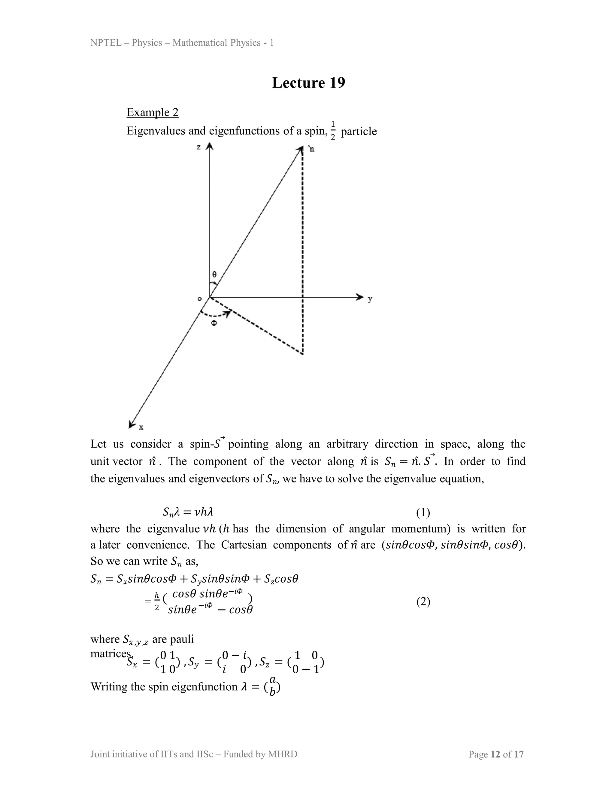
This document discusses finding the eigenvalues and eigenfunctions of a spin-1/2 particle pointing along an arbitrary direction. It shows that the eigenvalue equation reduces to a set of two linear, homogeneous equations. The eigenvalues are found to be ±1/2, and the corresponding eigenvectors are written in terms of the direction angles θ and Φ. As an example, it shows that for a spin oriented along the z-axis, the eigenvectors reduce to simple forms as expected for a spin-1/2 particle. It also introduces the Gauss elimination method for numerically solving systems of linear equations that arise in eigenvalue problems.