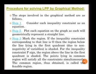
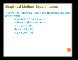
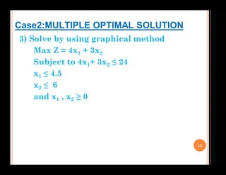
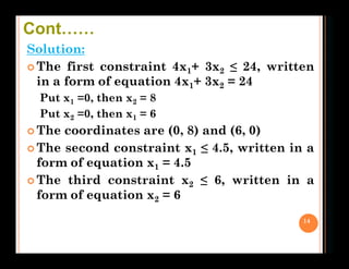
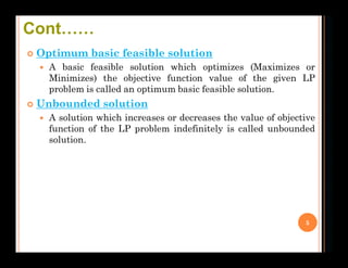
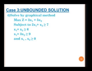
This document discusses different types of solutions that can arise when solving linear programming problems graphically: 1) A unique optimal solution occurs when the feasible region is bounded and the objective function is optimized at a single corner point. 2) Multiple optimal solutions arise if the objective function attains the same optimal value at multiple corner points. 3) An unbounded solution results when the feasible region is unbounded and the objective function can increase indefinitely. 4) No feasible solution exists if the constraints defining the feasible region are inconsistent and do not intersect, leaving an empty feasible region. Examples of each case are presented and solved graphically.

1. GRAPHICAL METHOD-SPECIAL CASES
1
C.Mohanraja, M Sc., MSc(M).,M Tech., MBA., MPhil.,
Assistant Professor in Computer Science,
St. Joseph’s College (Autonomous),
Tiruchirappallai-620 002.

2. Graphical Method-Special cases
Unique optimal solution
Multiple optimal solution
Unbound optimal solution
No feasible solution
2

3.  Feasible solution
 The set of values of decision variables Xj (j=1 2……n) which
satisfy all the constraints and non-negativity conditions of
an LP problem simultaneously is said to be the feasible
solution to that linear programming problem.
 Infeasible solution
 The set of values of decision variables Xj (j=1 2……n) which
do not satisfy all the constraints and non-negativity
conditions of an LP problem simultaneously is said to
constitute the infeasible solution to that linear
programming problem.
 Basic solution
 For a set of m simultaneous equations in n variables, a
solution obtained by setting (n-m) variables equal to zero
and solving for remaining m equations in m variables is
called a basic solutions.
3
Basic Definition:

4.  Non basic and basic variable
 The (n-m) variables whose values did not appear in this
solution are called non basic variable and the remaining m
variables are called basic variables.
 Basic feasible solution
 A feasible solution to an LP problem which is also the basic
solution is called the basic feasible solution. All basic
variables assume non-negative values.
Basic feasible solutions are of two types,
 (a) Degenerate: A basic feasible solution is called
degenerate if value of at least one basic variable is zero.
 (b) Non-degenerate: A basic feasible solution is called non-
degenerate if values all m basic variables are non-zero and
positive.
4
Cont……

5.  Optimum basic feasible solution
 A basic feasible solution which optimizes (Maximizes or
Minimizes) the objective function value of the given LP
problem is called an optimum basic feasible solution.
 Unbounded solution
 A solution which increases or decreases the value of objective
function of the LP problem indefinitely is called unbounded
solution.
5
Cont……

6.  The steps involved in the graphical method are as
follows.
 Step 1 Consider each inequality constraint as an
equation.
 Step 2 Plot each equation on the graph as each will
geometrically represent a straight line.
 Step 3 Mark the region. If the inequality constraint
corresponding to that line is O then the region below
the line lying in the first quadrant (due to non-
negativity of variables) is shaded. For the inequality
constraint P sign, the region above the line in the first
quadrant is shaded. The points lying in common
region will satisfy all the constraints simultaneously.
The common region, thus obtained, is called the
feasible region.
6
Procedure for solving LPP by Graphical Method:

7.  Step 4 Assign an arbitrary value, say zero, for the
objective function.
 Step 5 Draw a straight line to represent the objective
function with the arbitrary value (i.e., a straight line
through the origin).
 Step 6 Stretch the objective function line till the
extreme points of the feasible region. In the
maximization case, this line will stop farthest from the
origin, passing through at least one corner of the feasible
region. In the minimization case, this line will stop
nearest to the origin and passes through at least one
corner of the feasible region.
 Step 7 Find the coordinates of the extreme points
selected in step 6 and find the maximum or minimum
value of Z.
7
Cont……

8. 1)Solve the following linear programming problem
graphically:
Maximise Z = 4x + y ... (1)
subject to the constraints:
x + y ≤ 50 ... (2)
3x + y ≤ 90 ... (3)
x ≥ 0, y ≥ 0 ... (4)
8
Graphical Method-Special cases

9. Solution:
 The shaded region in Fig 1 is the feasible region
determined by the system of constraints (2) to (4).
 We observe that the feasible region OABC is bounded.
So, we now use Corner Point Method to determine the
maximum value of Z.
 The coordinates of the corner points O, A, B and C are
(0, 0), (30, 0), (20, 30) and (0, 50) respectively.
9
Cont……

10.  Now we evaluate Z at each corner point.
 Hence, maximum value of Z is 120 at the point (30, 0).
10
Fig A
Cont……

11. 1)Solve the following linear programming problem
graphically:
Minimise Z = 200 x + 500 y ... (1)
subject to the constraints:
x + 2y ≥ 10 ... (2)
3x + 4y ≤ 24 ... (3)
and x ,y ≥ 0 ... (4)
11
Case 1:UNIQUE OPTIMAL SOLUTION

12.  The shaded region in Fig B is the feasible region ABC
determined by the system of constraints (2) to (4), which
is bounded.
 The coordinates of corner points A, B and C are (0,5),
(4,3) and (0,6) respectively.
 Now we evaluate Z = 200x + 500y at these points.
Hence, minimum value of
Z is 2300 attained at
the unique point (4, 3) . 12
Solution
Fig B

13. 13
Case2:MULTIPLE OPTIMAL SOLUTION
3) Solve by using graphical method
Max Z = 4x1 + 3x2
Subject to 4x1+ 3x2 ≤ 24
x1 ≤ 4.5
x2 ≤ 6
and x1 , x2 ≥ 0

14. Solution:
 The first constraint 4x1+ 3x2 ≤ 24, written
in a form of equation 4x1+ 3x2 = 24
Put x1 =0, then x2 = 8
Put x2 =0, then x1 = 6
 The coordinates are (0, 8) and (6, 0)
 The second constraint x1 ≤ 4.5, written in a
form of equation x1 = 4.5
 The third constraint x2 ≤ 6, written in a
form of equation x2 = 6
14
Cont……

15.  The corner points of feasible region are A, B, C and D.
 Max Z = 24, which is achieved at both B and C corner
points. It can be achieved not only at B and C but every
point between B and C.
 Hence the given problem has multiple optimal solutions.
15
Cont…… Corner points Corresponding
value of Z= 4x1 + 3x2
A (0, 6)
B (1.5, 6)-
(Solve the two
equations 4x1+ 3x2 =
24 and x2 = 6 to get
the coordinates)
C (4.5, 2)-
(Solve the two
equations 4x1+ 3x2 =
24 and x1 = 4.5 to get
the coordinates)
D (4.5, 0)
Z = 4(0) + 3(6) = 18
Z = 4(1.5) + 3(6) = 24
Z = 4(4.5) + 3(2) = 24
Z = 4(4.5) + 3(0) = 18

16. 4)Solve by graphical method
Max Z = 3x1 + 5x2
Subject to 2x1+ x2 ≥ 7
x1+ x2 ≥ 6
x1+ 3x2 ≥ 9
and x1 , x2 ≥ 0
16
Case 3:UNBOUNDED SOLUTION

17. Solution:
 The first constraint 2x1+ x2 ≥ 7, written in a form
of equation 2x1+ x2 = 7
Put x1 =0, then x2 = 7
Put x2 =0, then x1 = 3.5
The coordinates are (0, 7) and (3.5, 0)
 The second constraint x1+ x2 ≥ 6, written in a
form of equation x1+ x2 = 6
Put x1 =0, then x2 = 6
Put x2 =0, then x1 = 6
The coordinates are (0, 6) and (6, 0) 17
Cont……

18. 18
Cont……
 The third constraint x1+ 3x2 ≥ 9, written in a form of
equation x1+ 3x2 = 9
Put x1 =0, then x2 = 3
Put x2 =0, then x1 = 9 The coordinates are (0, 3) and (9, 0)
Toordinates for the corner points
Corner points Corresponding
value of
Z = 3x1 + 5x2
A (0, 7)
B (1, 5) (Solve the
two equations
2x1+ x2 = 7 and
x1+ x2 = 6 to get
the coordinates)
C (4.5, 1.5) (Solve
the two equations
x1+ x2 = 6 and x1+
3x2 = 9 to get the
coordinates)
D (9, 0)
Z = 3(0) + 5(7) =
35
Z = 3(1) + 5(5) =
28
Z = 3(4.5) + 5(1.5)
= 21
Z = 3(9) + 5(0) =
27

19.  The corner points of feasible region are A, B, C
and D.
 The values of objective function at corner points
are 35, 28, 21 and 27.
 But there exists infinite number of points in the
feasible region which is unbounded.
 The value of objective function will be more
than the value of these four corner points i.e.
the maximum value of the objective function
occurs at a point at ∞.
 Hence the given problem has unbounded
solution. 19
Cont……

20. 20
5)Solve graphically
Max Z = 3x1 + 2x2
Subject to
x1+ x2 ≤ 1
x1+ x2 ≥ 3
and x1 , x2 ≥ 0
Case 4:NO FEASIBLE SOLUTION

21. Solution
 The first constraint x1+ x2 ≤ 1, written in a
form of equation x1+ x2 = 1
Put x1 =0, then x2 = 1
Put x2 =0, then x1 = 1
The coordinates are (0, 1) and (1, 0)
 The first constraint x1+ x2 ≥ 3, written in a
form of equation x1+ x2 = 3
Put x1 =0, then x2 = 3
Put x2 =0, then x1 = 3
The coordinates are (0, 3) and (3, 0)
21
Cont……

22.  There is no common feasible region generated by two
constraints together i.e. we cannot identify even a
single point satisfying the constraints.
 Hence there is no feasible solution. 22
Cont……

23. Thank You
23