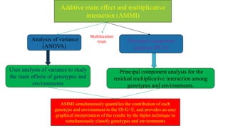
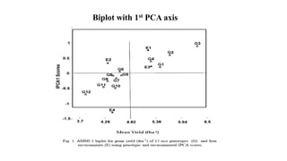
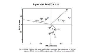
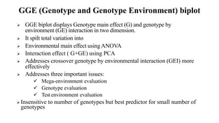
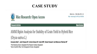
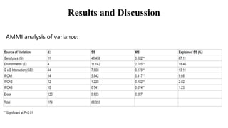
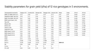
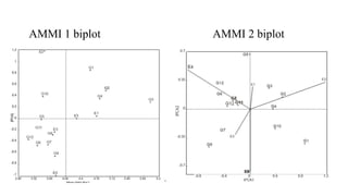
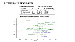
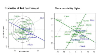
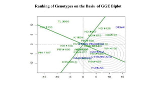
Selection Systems-Biplots and Mapping Genotypes
Submitted to:
Dr. K.B.ESWARI
PROFESSOR
Dept of Genetics and Plant breeding
Submitted by:
ANIL KUMAR
RAM/2020-68
Dept pf Genetics and Plant Breeding
Biplot
A biplot is a scatter plot that graphically displays both the row factors and
the column factors of a two-way data.
A biplot allows information on both samples and variables of a data
matrix to be displayed graphically.
 Samples are displayed as points while variables are displayed either as
vectors, linear axes or nonlinear trajectories.
This technique has extensively been used in the analysis of multi-
environment trials.
The biplot was introduced by K. Ruben Gabriel (1971).
Construction of biplots
Biplots constructed with the help of-
 The additive main effect and multiplicative interaction
(AMMI) method
Analysis of variance (ANOVA) and principal component
analysis (PCA) into a unified approach that can be used
to analyze multi-location trials.
Additive main effect and multiplicative
interaction (AMMI)
Analysis of variance
(ANOVA)
Principal component
analysis (PCA)
Uses analysis of variance to study
the main effects of genotypes and
environments
Principal component analysis for the
residual multiplicative interaction among
genotypes and environments.
AMMI simultaneously quantifies the contribution of each
genotype and environment to the SS-G×E, and provides an easy
graphical interpretation of the results by the biplot technique to
simultaneously classify genotypes and environments
Multilocation
trials
Principal components:
 The first principal component (PC1) represents responses of the genotypes
that are proportional to the environments, which are associated with the GxE
interaction.
 The second principal component (PC2) provides information about
cultivation locations that are not proportional to the environments, indicating
that those are responsible of the GxE crossover interaction.
Feature of PCA:
• It computes a genotype score and an environment score whose product
estimate yield for that genotype in that environment .
1.Biplot with First PCA Axis
A biplot is developed by placing both genotype and environmental mean (main effect) on x-axis and representing
PCA axis eigen vector on the y-axis
The biplot helps to visualize relationship between eigen values for PCA1 and genotypic and environmental
means.
If a genotype or an environment has a IPCA1 score of nearly zero, it has small interaction effects and considered
as stable.
When a genotype and environment have the same sign on the PCA axis, their interaction is positive and if
different, their interaction is negative.
Two kinds of plotting is possible with estimatedAMMI interaction parameters
Biplot with 1st PCA axis
For a better description of the interaction, both first and second PCA scores of genotypes and
environments may be considered for plotting.
Here IPCA 2 score of genotypes and environments are plotted against their respective IPCA 1
score.
The environmental scores are joined to the origin by side lines. Sites with short spokes do not
exert strong interactive forces. Those with long spokes exert strong interaction.
The genotypes occurring close together on the plot will tend to have similar yields in all
environments, while genotypes far apart show a different pattern of response over the
environments.
Hence, the genotypes near the origin are not sensitive to environmental interaction and those
distant from the origins are sensitive and have large interaction.
2. Biplot with Two PCA Axis
Biplot with Two PCA Axis
GGE (Genotype and Genotype Environment) biplot
 GGE biplot displays Genotype main effect (G) and genotype by
environment (GE) interaction in two dimension.
 It spilt total variation into
 Environmental main effect using ANOVA
 Interaction effect ( G+GE) using PCA
 Addresses crossover genotype by environmental interaction (GEI) more
effectively
 Addresses three important issues:
 Mega-environment evaluation
 Genotype evaluation
 Test environment evaluation
 Insensitive to number of genotypes but best predictor for small number of
genotypes
MOLECULAR MAPPING
The chief breeding objective served by molecular marker is
identification of markers tightly linked to genes contributing to
desirable phenotype.
This would allow indirect selection on the basis of linked markers.
In order to realize the objective, molecular markers linked to the gene
of interest need to be identified.
There are two approaches for achieving this:
Association mapping
Linkage mapping
Mapping of Quantitative Trait Loci (QTLs)
 The process of constructing linkage maps and conducting QTL
analysis i.e. to identify genomic regions associated with traits is
known as QTL mapping.
 Identification and location of polygenes or QTL by use of DNA
markers.
 It involves testing DNA markers throughout the genome for the
likelihood that they are associated with a QTL.
Prerequisites for QTL mapping
A suitable mapping Population (population Size 50 to 250
individuals)
A dense marker linkage Map
A reliable phenotypic evaluation for target trait.
Software available for analysis- Mapmaker/EXP , MapManager
QTX, Joinmap etc.
Sophisticated Laboratory
Steps in QTL Mapping
 DEVELOPMENT OF LINKAGE MAP
1. Creation of suitable mapping population
2. Phenotyping of mapping population.
3. Identification of molecular marker that differ between two parents i.e.,
polymorphic.
4. Genotyping of mapping population
5. Construction of linkage map using data generated from genotyping and
phenotyping.
 DETECTION OF QTLs
Mapping populations
 A population that is suitable for linkage mapping of genetic markers.
 F2 population
 F2 derived F3 population
 Backcross
 Doubled haploids
 Recombinant inbred lines
 Near isogenic lines
 Backcross inbred lined
Construction of linkage map
Data generated by genotyping and phenotyping are subjected to linkage
analysis using suitable Software such as ‘Mapmaker/EXP’, ‘MapManager
QTX’ or ‘Joinmap’.
The computer programmes detect linkage by computation of LOD
(logarithm of odds) score.
If LOD score is 3.0 or more, it is considered that two markers are linked.
QTLAnalysis
It is based on the principle of detecting an association between
phenotype and the genotype of the markers.
It is not easy to do this analysis manually and so with the help of a
computer and a software it is done.
The segregation data of both the phenotype and the genotype are
collected and arranged in an excel sheet for QTL analysis using the
appropriate software.
Methods to detect QTLs
 Single-marker analysis,
 Simple interval mapping and
 Composite interval mapping
 Multiple Interval Mapping
 Bayesian Interval Mapping
CASE STUDY
Objective:
To identify more high yielding stable promising hybrids and to determine
the areas where rice hybrids would be adapted by AMMI model.
Materials and Methods:
12 genotypes of Rice
5 Different environments :Gazipur(E1), Comilla (E2), Barisal (E3),
Rangpur (E4) and Jessore (E5)
Randomized complete block design (RCBD) with 3 Replications
Results and Discussion
AMMI analysis of variance:
Stability parameters for grain yield (t/ha) of 12 rice genotypes in 5 environments.
AMMI 1 biplot AMMI 2 biplot
Conclusions
The mean grain yield value of genotypes averaged over environments
indicated that the genotypes G3 and G12 had the highest (5.99 tha-1) and the
lowest (3.19 tha-1) yield, respectively.
It is noted that the variety G3 showed higher grain yield than all other
varieties over all the environments.
The hybrids (G1), (G2), (G3) and (G4) were hardly affected by the G x E
interaction and thus will perform well across a wide range of environments.
Objective
To study the construction and application of GGE biplots for interpretation of
genotype versus environment interactions data for wheat yield in Northern India.
MATERIALS AND METHODS
23 genotypes of wheat
6 environments/states of Northern India (Delhi, Uttar Pradesh, Haryana,
Uttarakhand, Punjab and Rajasthan)
Randomised complete block design
GGE Biplot Analysis
RESULTS AND DISCUSSION
Differentiation of Genotypes in GGE biplot
Analysis of variance of G × E data for North India
Differentiation of environments in GGE biplot Mega-environments Analysis
Evaluation of Test Environment Mean vs stability Biplot
Ranking of Genotypes on the Basis of GGE Biplot
CONCLUSIONS
Genotype pairs such as (TL2995, PBW697), (HD3128, WH1157) and (WH1157,
DBW95) were found to be dissimilar while WH1138, PBW681 and PBW677 were
observed to be the most similar genotypes
Haryana environment having the smallest angle had the highest representativeness
while Rajasthan with the largest angle had the lowest representation.
Delhi environment was observed to be the most discriminating while Uttar Pradesh as
the least discriminating.
The genotype WH1105 was observed to be the most favorable followed by PBW698
for North Zone of India
Selection system: Biplots and Mapping genotyoe

Selection system: Biplots and Mapping genotyoe

  • 1.
    Selection Systems-Biplots andMapping Genotypes Submitted to: Dr. K.B.ESWARI PROFESSOR Dept of Genetics and Plant breeding Submitted by: ANIL KUMAR RAM/2020-68 Dept pf Genetics and Plant Breeding
  • 2.
    Biplot A biplot isa scatter plot that graphically displays both the row factors and the column factors of a two-way data. A biplot allows information on both samples and variables of a data matrix to be displayed graphically.  Samples are displayed as points while variables are displayed either as vectors, linear axes or nonlinear trajectories. This technique has extensively been used in the analysis of multi- environment trials. The biplot was introduced by K. Ruben Gabriel (1971).
  • 4.
    Construction of biplots Biplotsconstructed with the help of-  The additive main effect and multiplicative interaction (AMMI) method Analysis of variance (ANOVA) and principal component analysis (PCA) into a unified approach that can be used to analyze multi-location trials.
  • 5.
    Additive main effectand multiplicative interaction (AMMI) Analysis of variance (ANOVA) Principal component analysis (PCA) Uses analysis of variance to study the main effects of genotypes and environments Principal component analysis for the residual multiplicative interaction among genotypes and environments. AMMI simultaneously quantifies the contribution of each genotype and environment to the SS-G×E, and provides an easy graphical interpretation of the results by the biplot technique to simultaneously classify genotypes and environments Multilocation trials
  • 6.
    Principal components:  Thefirst principal component (PC1) represents responses of the genotypes that are proportional to the environments, which are associated with the GxE interaction.  The second principal component (PC2) provides information about cultivation locations that are not proportional to the environments, indicating that those are responsible of the GxE crossover interaction. Feature of PCA: • It computes a genotype score and an environment score whose product estimate yield for that genotype in that environment .
  • 7.
    1.Biplot with FirstPCA Axis A biplot is developed by placing both genotype and environmental mean (main effect) on x-axis and representing PCA axis eigen vector on the y-axis The biplot helps to visualize relationship between eigen values for PCA1 and genotypic and environmental means. If a genotype or an environment has a IPCA1 score of nearly zero, it has small interaction effects and considered as stable. When a genotype and environment have the same sign on the PCA axis, their interaction is positive and if different, their interaction is negative. Two kinds of plotting is possible with estimatedAMMI interaction parameters
  • 8.
  • 9.
    For a betterdescription of the interaction, both first and second PCA scores of genotypes and environments may be considered for plotting. Here IPCA 2 score of genotypes and environments are plotted against their respective IPCA 1 score. The environmental scores are joined to the origin by side lines. Sites with short spokes do not exert strong interactive forces. Those with long spokes exert strong interaction. The genotypes occurring close together on the plot will tend to have similar yields in all environments, while genotypes far apart show a different pattern of response over the environments. Hence, the genotypes near the origin are not sensitive to environmental interaction and those distant from the origins are sensitive and have large interaction. 2. Biplot with Two PCA Axis
  • 10.
  • 11.
    GGE (Genotype andGenotype Environment) biplot  GGE biplot displays Genotype main effect (G) and genotype by environment (GE) interaction in two dimension.  It spilt total variation into  Environmental main effect using ANOVA  Interaction effect ( G+GE) using PCA  Addresses crossover genotype by environmental interaction (GEI) more effectively  Addresses three important issues:  Mega-environment evaluation  Genotype evaluation  Test environment evaluation  Insensitive to number of genotypes but best predictor for small number of genotypes
  • 12.
    MOLECULAR MAPPING The chiefbreeding objective served by molecular marker is identification of markers tightly linked to genes contributing to desirable phenotype. This would allow indirect selection on the basis of linked markers. In order to realize the objective, molecular markers linked to the gene of interest need to be identified. There are two approaches for achieving this: Association mapping Linkage mapping
  • 13.
    Mapping of QuantitativeTrait Loci (QTLs)  The process of constructing linkage maps and conducting QTL analysis i.e. to identify genomic regions associated with traits is known as QTL mapping.  Identification and location of polygenes or QTL by use of DNA markers.  It involves testing DNA markers throughout the genome for the likelihood that they are associated with a QTL.
  • 14.
    Prerequisites for QTLmapping A suitable mapping Population (population Size 50 to 250 individuals) A dense marker linkage Map A reliable phenotypic evaluation for target trait. Software available for analysis- Mapmaker/EXP , MapManager QTX, Joinmap etc. Sophisticated Laboratory
  • 15.
    Steps in QTLMapping  DEVELOPMENT OF LINKAGE MAP 1. Creation of suitable mapping population 2. Phenotyping of mapping population. 3. Identification of molecular marker that differ between two parents i.e., polymorphic. 4. Genotyping of mapping population 5. Construction of linkage map using data generated from genotyping and phenotyping.  DETECTION OF QTLs
  • 16.
    Mapping populations  Apopulation that is suitable for linkage mapping of genetic markers.  F2 population  F2 derived F3 population  Backcross  Doubled haploids  Recombinant inbred lines  Near isogenic lines  Backcross inbred lined
  • 17.
    Construction of linkagemap Data generated by genotyping and phenotyping are subjected to linkage analysis using suitable Software such as ‘Mapmaker/EXP’, ‘MapManager QTX’ or ‘Joinmap’. The computer programmes detect linkage by computation of LOD (logarithm of odds) score. If LOD score is 3.0 or more, it is considered that two markers are linked.
  • 18.
    QTLAnalysis It is basedon the principle of detecting an association between phenotype and the genotype of the markers. It is not easy to do this analysis manually and so with the help of a computer and a software it is done. The segregation data of both the phenotype and the genotype are collected and arranged in an excel sheet for QTL analysis using the appropriate software.
  • 19.
    Methods to detectQTLs  Single-marker analysis,  Simple interval mapping and  Composite interval mapping  Multiple Interval Mapping  Bayesian Interval Mapping
  • 20.
  • 21.
    Objective: To identify morehigh yielding stable promising hybrids and to determine the areas where rice hybrids would be adapted by AMMI model. Materials and Methods: 12 genotypes of Rice 5 Different environments :Gazipur(E1), Comilla (E2), Barisal (E3), Rangpur (E4) and Jessore (E5) Randomized complete block design (RCBD) with 3 Replications
  • 22.
    Results and Discussion AMMIanalysis of variance:
  • 23.
    Stability parameters forgrain yield (t/ha) of 12 rice genotypes in 5 environments.
  • 24.
    AMMI 1 biplotAMMI 2 biplot
  • 25.
    Conclusions The mean grainyield value of genotypes averaged over environments indicated that the genotypes G3 and G12 had the highest (5.99 tha-1) and the lowest (3.19 tha-1) yield, respectively. It is noted that the variety G3 showed higher grain yield than all other varieties over all the environments. The hybrids (G1), (G2), (G3) and (G4) were hardly affected by the G x E interaction and thus will perform well across a wide range of environments.
  • 27.
    Objective To study theconstruction and application of GGE biplots for interpretation of genotype versus environment interactions data for wheat yield in Northern India. MATERIALS AND METHODS 23 genotypes of wheat 6 environments/states of Northern India (Delhi, Uttar Pradesh, Haryana, Uttarakhand, Punjab and Rajasthan) Randomised complete block design GGE Biplot Analysis
  • 28.
    RESULTS AND DISCUSSION Differentiationof Genotypes in GGE biplot Analysis of variance of G × E data for North India
  • 29.
    Differentiation of environmentsin GGE biplot Mega-environments Analysis
  • 30.
    Evaluation of TestEnvironment Mean vs stability Biplot
  • 31.
    Ranking of Genotypeson the Basis of GGE Biplot
  • 32.
    CONCLUSIONS Genotype pairs suchas (TL2995, PBW697), (HD3128, WH1157) and (WH1157, DBW95) were found to be dissimilar while WH1138, PBW681 and PBW677 were observed to be the most similar genotypes Haryana environment having the smallest angle had the highest representativeness while Rajasthan with the largest angle had the lowest representation. Delhi environment was observed to be the most discriminating while Uttar Pradesh as the least discriminating. The genotype WH1105 was observed to be the most favorable followed by PBW698 for North Zone of India