This document discusses quantitative trait loci (QTL) mapping. It begins by defining QTLs as genomic regions containing genes associated with quantitative traits. QTL mapping involves correlating genotypic and phenotypic data from a mapping population to identify these regions. Common mapping populations discussed include recombinant inbred lines, double haploids, and backcrosses. Interval mapping and composite interval mapping are presented as methods for QTL analysis. The goals of QTL mapping are to locate genomic regions influencing traits and estimate the effects of QTLs.

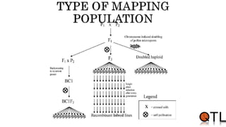
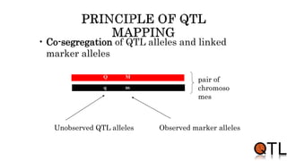
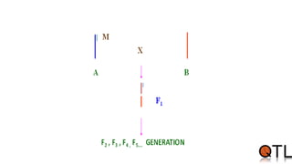
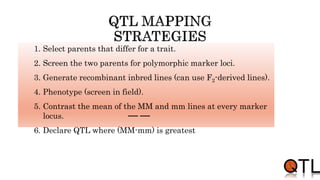
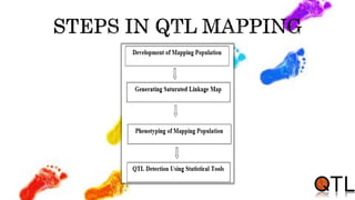
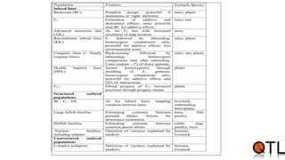
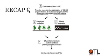
1. PRESENTED BY,
SANDESH,G.M
2016610811
TNAU. MADURAI

3.  Generally single gene trait
 No environmental influence
 Presence or absence
• Growth habit: Tall vs. Dwarf
• Pigmentation:
Pigmented vs. Non-pigmented
• Disease reaction:
Resistant vs. susceptible

4.  Generally more than one gene.
 Environmental effects.
 Quantity:
• Tillers
• Yield
Phenotype = Genotype + Environment + Management

5.  Correlate segregation of the quantitative trait with that of
qualitative trait, i.e., markers
QTL = Quantitative Trait Locus = GENE

6.  Locus, meaning region of the genome –
not necessarily a single gene, could be several linked genes.
 QTL is a region of the genome that contain gene(s)associated with a
quantitative trait.
 Allelic variation at a QTL region causes phenotypic variation in a
quantitative trait.
 It is coined by Gelderman .

7.  A variety may have some QTL that increase a trait (for example,
increase yield) and others that decrease the trait. These work
together to create the phenotype of the plant.
In this example genome have 3 loci, one associated with decreased yield,
and one associated with higher yield. The phenotype, depending on the size of
the effect of each QTL and how they work together, may be low yield.

8. The key is identifying the “good” QTL – Those that affect the trait
in the direction you want, and then separating those from the
negative ones. This is where QTL identification techniques are
important. e.g.
Positive QTL: Grain Yield, Disease resistance, Oil content, Protein or
Mineral linked.
Negative QTL: Plant Height, Environment effected traits.
Note that these techniques are simply statistical correlations, just
like genetic mapping and any marker-trait correlations; however,
because we are looking for many markers that correlate with a
single trait, it is somewhat more complex statistically.

9. The process of constructing linkage maps and conducting QTL analysis–to
identify genomic regions associated with traits–is known as QTL mapping
(McCouch & Doerge, 1995).
A QTL map is the correlation of genotypic data of individuals from
mapping population with phenotypic information
Phenotype data + linkage map = QTLs

10.  Identify regions of the genome containing QTLs.
 Estimate the effects of the QTLs on the quantitative trait:
1.how much of the variation for the trait is caused by a specific
region?
2.what is the gene action associated with the QTL – additive
effect?
3.Dominant effect?
4.which allele is associated with the favourable effect?

12.  Availability of a good linkage map (this can be done at the same time
the QTL mapping).
 A segregating population derived from parents that differ for the
trait(s) of interest, and which allow for replication of each segregant,
so that phenotype can be measured with precision (such as RILs or
DHs).
 A good assay for the trait(s) of interest.
 Software available for analyses.

13. Backcrosses
F2 intercrosses
Recombinant inbred (RI) lines
Double Haploids

15. • Co-segregation of QTL alleles and linked
marker alleles
Unobserved QTL alleles
q m
Q M
Observed marker alleles
pair of
chromoso
mes

17. 1. Select parents that differ for a trait.
2. Screen the two parents for polymorphic marker loci.
3. Generate recombinant inbred lines (can use F2-derived lines).
4. Phenotype (screen in field).
5. Contrast the mean of the MM and mm lines at every marker
locus.
6. Declare QTL where (MM-mm) is greatest

19. Population Features Example Species
Inbred lines
Backcross (BC) Simplest design; powerful if
dominance in ‘right’ direction
mice, plants
F2 Estimation of additive and
dominance effects; more powerful
than BC for additive effects
mice, rats
Advanced intercross line
(AIL)
As for F2 but with increased
resolution of map location
mice
Recombinant inbred lines
(RIL)
F1 followed by inbreeding;
homozygous comparisons only;
powerful for additive effects; less
environmental noise
mice, plants
Congenic lines (= Nearly
isogenic lines)
Backcrossing followed by
inbreeding; homozygous
comparisons only after inbreeding.
Lines contain ~1% of donor genome
mice, rats, plants
Double haploid lines
(DHL)
Instant homozygosity through
doubling of F1 gametes;
homozygous comparisons only;
powerful for additive effects and
QTLxE interactions
plants
F2:3 Inbred progeny of F2; increased
precision through progeny means
plants
Structured outbred
populations
BC / F2 / AIL As for inbred lines; mapping
variation between lines
livestock,
outbreeding
trees/plants
Large fullsib families Estimating contrasts between
parental alleles. Allows for
dominance estimation.
trees, fish,
poultry
Halfsib families Estimating contrasts between
common parent alleles
cattle, pigs,
poultry, trees
Nuclear families,
including sibpairs
Detection of variance explained by
markers
humans,
livestock
Unstructured outbred
populations
Complex pedigrees Detection of variance explained by
markers
humans,
livestock

20.  In large sample size, QTL with small effects can not be observed but
QTL with large effects can be observed.
 In small sample size also, QTL with small effects can not be observed
but QTL with major effects can be observed.

21.  Number of markers used - estimation of both QTL position and effect.
 co-dominant marker shows three types of genetic difference while
dominant marker shows two types of genetic difference.

24.  QTL Data is typically pooled over locations and replications to obtain
a single quantitative trait for the line.
 It is also preferred to measure the target trait(s) in experiments
conducted in multiple (and appropriate) locations to have a better
understanding of the QTL x environment interaction, if any.

26.  DNA markers can be used to map useful genes using recombination
frequencies of linked genes:
A
a
M
m
QTL Marker
• Markers near QTLs co-segregate with them.
• Markers tightly linked to QTL detected by ANOVA.
• Most gametes from this F1 = AM or am. If crossover between marker &
QTL, Am & aM gametes will be produced.

27. 1. Select parents that differ for a trait.
2. Screen the two parents for polymorphic marker loci.
3. Generate recombinant inbred lines (can use F2-derived lines).
4. Phenotype (screen in field).
5. Do a separate ANOVA on the effect of each marker.
6. Declare QTL where F-test is significant.
This technique is good choice when the goal is simple detection of a QTL linked
to a marker, rather than estimation of its position and effects.

28.  This method cannot determine whether the
markers are associated with one or more
QTLs.
 Chance of QTL detection decreases with
distance between marker and QTL.
 Its accuracy is less .

29.  Lander & Botstein (1989).
• Analyzes intervals between adjacent markers instead of single
markers.
• Statistically more powerful.
• Takes proper account of missing data.
• Gives improved estimates of QTL effects.
• Provides pretty graphs.
• Assume a single QTL model.
M1 A
m1 a
M2
m2

30. • Marker interval = the segment between 2 markers
• Interval mapping methods use information on values of 2 flanking
markers to estimate QTL position
• The probability that the data could be obtained assuming a QTL at
several positions between the markers is calculated.
• QTL = declared where the probability of obtaining the observed data is
highest.

31. • LOD of 2 means that it is 100x more likely that a QTL exists in the interval
than that there is no QTL.
• LOD of 3 means that it is 1000x more likely.
Significance test:
 Logarithm of the odds ratio (LOD score):
Probability of the data occurring with a QTL
Odds ratio =
Probability of the data occurring with no QTL

32.  Analyzes intervals between adjacent markers+ additional markers
unlinked to the interval markers to focus on the interval and
eliminate confounding effects from other QTLs
 Jansen and Stam (1994)
M1 A
m1 a
M2
m2
M3 B
m3 b
M4
m4

33.  CIM evaluates the possibility of a target QTL at multiple analysis points across each
inter-marker interval (same as SIM). However at each point it also includes the effect of
one or more background markers.
 Background markers: That have been shown to be associated with the trait and
therefore lie close to other QTLs (background QTLs) affecting the trait.
 The inclusion of a background marker in the analysis helps in one of two ways,
Based upon the linkage of Background marker and the target interval
1) If they are linked, inclusion of the background marker may help to separate the
target QTL from other linked QTLs.
2) If they are not linked, inclusion of the background marker makes the analysis more
sensitive to the presence of a QTL in the target interval.

34.  It is used to minimize effects of various linked QTLs.
 It is based on one QTL and other markers used as covariates.
 This technique gives more precise results and used to exclude bias
due to another QTLs (non-target QTLs) linked to target QTL.
 The partial regression coefficient is used to determine genetic
variance due to non-target QTLs.

35.  Mapping of multiple QTLs
 Increasing the precision of QTL mapping.
 By eliminating as much as the genetic variance produced by other
QTL - residual variance is reduced - efficiency of determination of
QTL is increased.
 CIM is more efficient than SIM, but not widely used in QTL mapping
as in SIM.

36.  Intense computation.
 Rely on a genetic map with good quality.
 Difficult to incorporate covariate.

37.  Recent method of QTL Mapping.
 Multiple Interval Mapping (MIM) is the extension of interval
mapping to multiple QTLs, just as multiple regression extends
analysis of variance.
 It is used to map multiple QTLs.
 This method is potential tool for detection of QTL X QTL interaction.

39.  The introgression of QTLs into elite lines / germplasm
 Maker-aided selection (MAS) for QTLs in crop improvement has to be
undertaken in some of the crop like
 Maize (Li et al.,2008),
 Tomato (Stevens et al., 2007)
 Wheat (Naz et al.,2008).
 QTLs so identified for diverse traits in different crops have been met in crop
improvement especially to enhance the yield and to develop disease
resistance elite lines.

42.  Number of genes controlling the target traits and their position.
 Heteritability of the genes segregating in a mapping population.
 Statistical tools.

43. The high quality phenotypic data is very important and useful for meaningful
genetic dissection and genomics-assisted breeding applications, including:
 QTL interval mapping
 Candidate-gene based association mapping
 Genome-wide association studies (GWAS)
 QTL cloning
 QTL meta-analysis
 Marker-assisted selection (MAS)
 Marker-assisted recurrent selection (MARS)
 TILLING (Targeting Induced Local Lesions in Genomes)and
 Genomic selection (GS) or genome-wide selection (GWS) (Welcker, 2011; Tuberosa
et al., 2012; Cobb et al., 2013;).

45. TISSUE CULTURE
A) Isolation, selection and handling of mature somatic embryos
• Development of visualisation and handling technology for
quality assessment, sorting and orientation of 3-5 mm long
mature embryos.
• Development of technologies for transfer of embryos to
germination medium.

47. B) Identification and transfer of germinated plants to soil
• Development of visualisation technology for identification of germinated plants
with root.
• Development of handling technologies for transfer of plants from sterile growth
medium to non sterile growth plugs.

48. ‘‘Motoman takes a novel approach to
increasing the productivity of automated
assays. (This includes) a compact work
cell equipped with washers, dispensers,
readers and incubators, serviced by a
multitude of plate handlers

51. A robot system for phenotyping large tomato plants in the
greenhouse using a 3D light field camera

53. Angaji S.A., QTL Mapping: A Few Key points. International Journal of Applied
Research in Natural Products, 2(2), 1-3 (2009)
Basten, C., B. Weir and Z.-B. Zeng, 2001. QTL cartographer. Department of
Statistics, North Carolina State University, Raleigh, NC.
Bernardo, R. 2002. Breeding for quantitative traits in plants. Chapters 13 and
14
Collard B.C.Y., Jahufer M.Z.Z., Brouwer J.B. and Pang E.C.K., An introduction
to markers, quantitative trait loci (QTL) mapping and marker-assisted
selection for crop improvement: The basic concepts, Euphytica 142, 169–196
(2005)
Davierwala A., Chowdari K., Kumar S., Reddy A., Ranjekar P. and Gupta V.,
Use of three different marker systems to estimate genetic diversity of Indian
elite rice varieties, Genetica 108, 269–284 (2000)
Kearsey, M.J. and Pooni, H.S. 1996. The genetical analysis of quantitative
traits. Chapter 7

54. THANK YOU..,