Downloaded 53 times
![8 ■
APPLICATIONS OF SECOND-ORDER DIFFERENTIAL EQUATIONS
Answers
x 12 kg 1
5 e6t 6
S Click here for solutions.
1. 3. 5.
7.
c=10
c=15
0 1.4
c=25
Qt e10t2506 cos 20t 3 sin 20t 3
13. ,
It 3
5 e10t sin 20t
Qt e10t[ 3
15.
3
250 cos 20t 3
500 sin 20t]
250 cos 10t 3
125 sin 10t
125
c=30
c=20
0.02
_0.11
49
x 0.36 sin10t3 5 et](https://image.slidesharecdn.com/app2odestewart1-140916200405-phpapp01/75/applications-of-second-order-differential-equations-8-2048.jpg)
![10 ■ APPLICATIONS OF SECOND-ORDER DIFFERENTIAL EQUATIONS
11. From Equation 6, x(t) = f(t) + g(t) where f(t) = c1 cos ωt + c2 sin ωt and g(t) =
F0
m(ω2 − ω20
)
cos ω0t. Then
f is periodic, with period 2π
ω , and if ω6= ω0, g is periodic with period 2π
ω0
. If ω
ω0
is a rational number, then we can
say ω
ω0
= a
b ⇒ a = bω
ω0
where a and b are non-zero integers. Then
¡
t + a · 2π
x
ω
¢
= f
¡
t + a · 2π
ω
¢
+ g
¡
t + a · 2π
ω
¢
= f(t) + g
³
t + bω
ω0 · 2π
ω
´
= f(t) + g
³
t + b · 2π
ω0
´
= f(t) + g(t) = x(t)
so x(t) is periodic.
13. Here the initial-value problem for the charge is Q00 + 20Q0 + 500Q = 12,
Q(0) = Q0(0) = 0. Then
Qc(t) = e−10t(c1 cos 20t + c2 sin 20t) and try Qp (t) = A ⇒ 500A = 12 or A = 3
125 .
The general solution is Q(t) = e−10t(c1 cos 20t + c2 sin 20t) + 3
125. But 0 = Q(0) = c1 + 3
125 and
Q0(t) = I(t) = e−10t[(−10c1 + 20c2) cos 20t + (−10c2 − 20c1) sin20t] but 0 = Q0(0) = −10c1 + 20c2. Thus
¡ ¢
the charge is Q(t) = − 1
e−10t(6 cos 20t + 3sin20t) + 3
and the current is I(t) = e−10t3
sin 20t.
250 125 5
15. As in Exercise 13, Qc(t) = e−10t(c1 cos 20t + c2 sin 20t) but E(t) = 12sin10t so try
Qp(t) = Acos 10t + B sin 10t. Substituting into the differential equation gives
(−100A +200B + 500A) cos10t + (−100B − 200A+ 500B) sin10t = 12sin10t ⇒ 400A +200B = 0
and 400B − 200A = 12. Thus A = − 3
, B = 3
and the general solution is
250 125 Q(t) = e−10t(c1 cos 20t + c2 sin 20t) − 3
250 cos 10t + 3
125 sin 10t. But 0 = Q(0) = c1 − 3
250 so c1 = 3
250 .
Also Q0(t) = 3
25 sin 10t + 6
25 cos 10t + e−10t[(−10c1 + 20c2) cos 20t + (−10c2 − 20c1) sin20t] and
0 = Q0(0) = 6
25 − 10c1 + 20c2 so c2 = − 3
500 . Hence the charge is given by
Q(t) = e−10t£ 3
250 cos 20t − 3
500 sin 20t
¤
− 3
250 cos 10t + 3
125 sin 10t.
³ c1
A
17. x(t) = Acos(ωt + δ) ⇔ x(t) = A[cos ωt cos δ − sin ωt sin δ] ⇔ x(t) = A
cos ωt +
c2
A
sin ωt
´
22
where cos 21
δ = c1/A and sin δ = −c2/A ⇔ x(t) = c1 cos ωt + c2 sin ωt. (Note that cos2 δ + sin2 δ = 1 ⇒
c+ c= A2.)](https://image.slidesharecdn.com/app2odestewart1-140916200405-phpapp01/75/applications-of-second-order-differential-equations-10-2048.jpg)

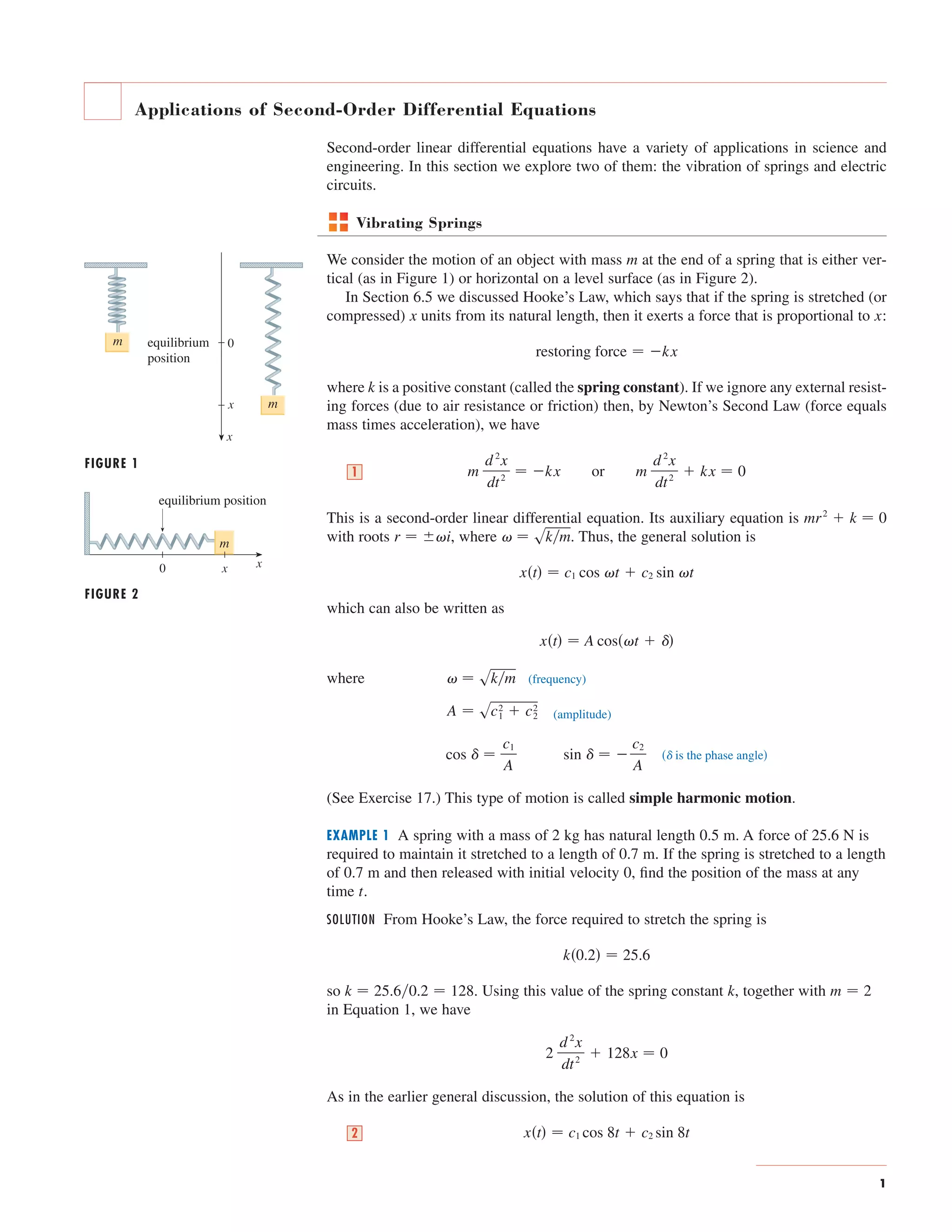
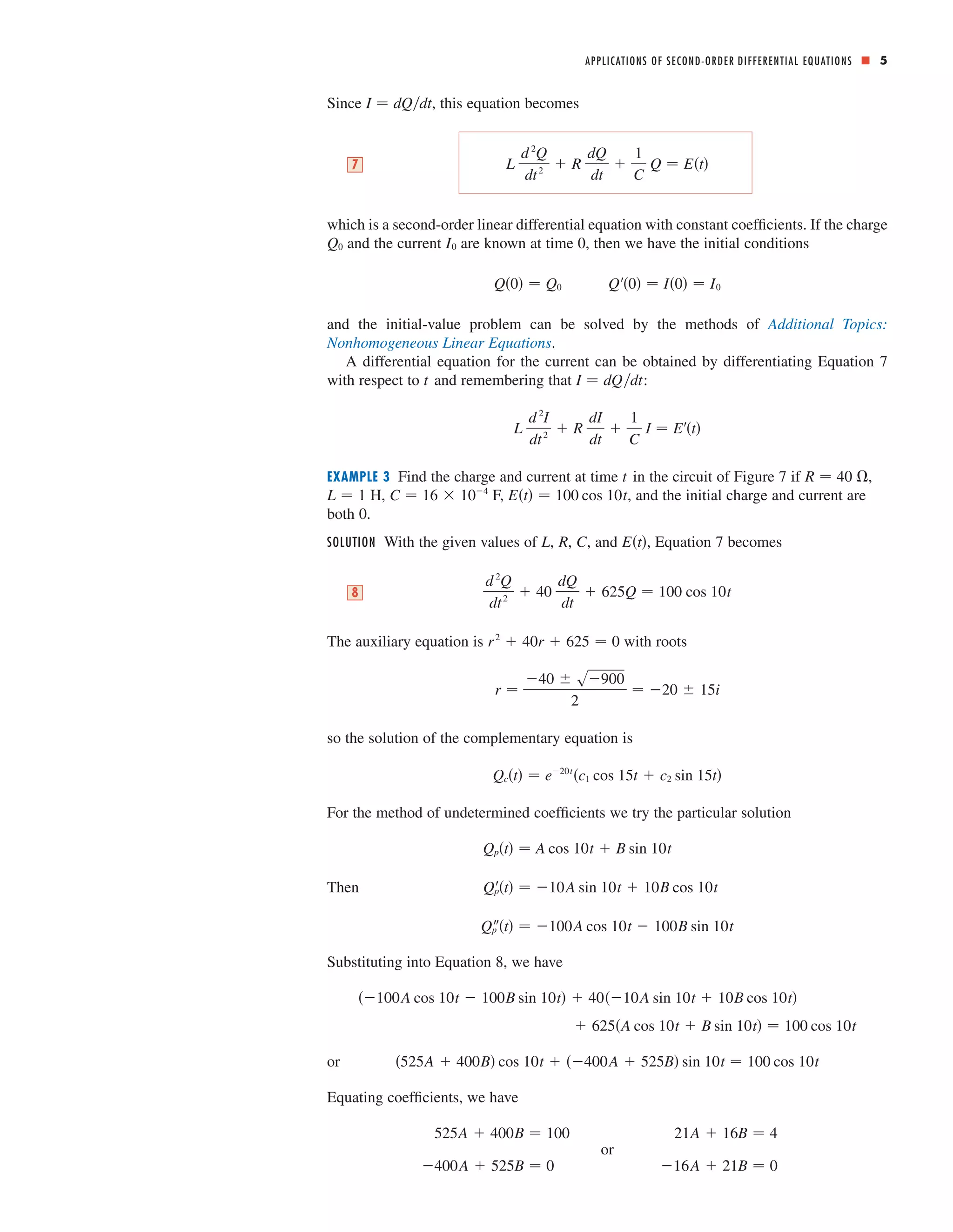
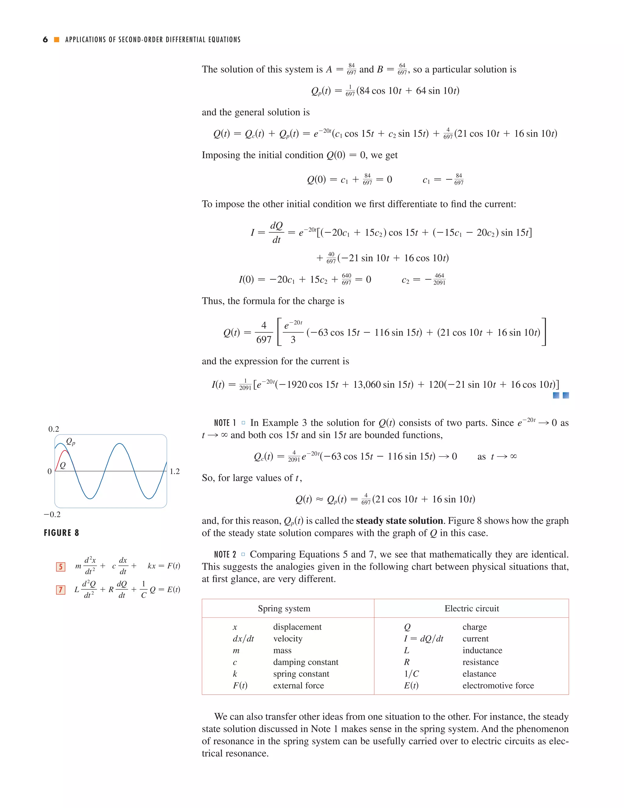
1) Second-order differential equations are used to model vibrating springs and electric circuits. They describe oscillations, vibrations, and resonance. 2) Springs obey Hooke's law, resulting in a second-order differential equation relating position to time. The solutions describe simple harmonic motion. 3) Damping forces can be added, resulting in overdamped, critically damped, or underdamped systems with different behavior.
Focuses on second-order differential equations, specifically vibrations of springs and damped vibrations.
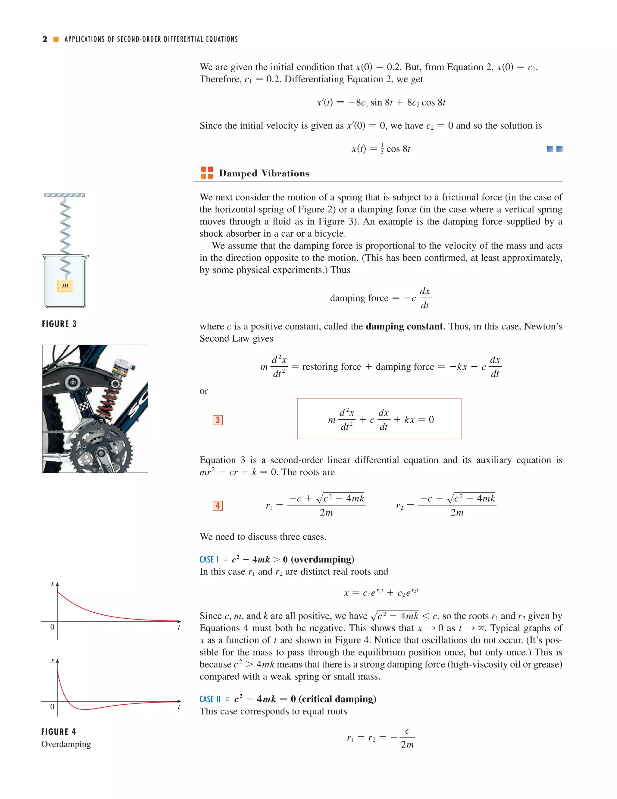
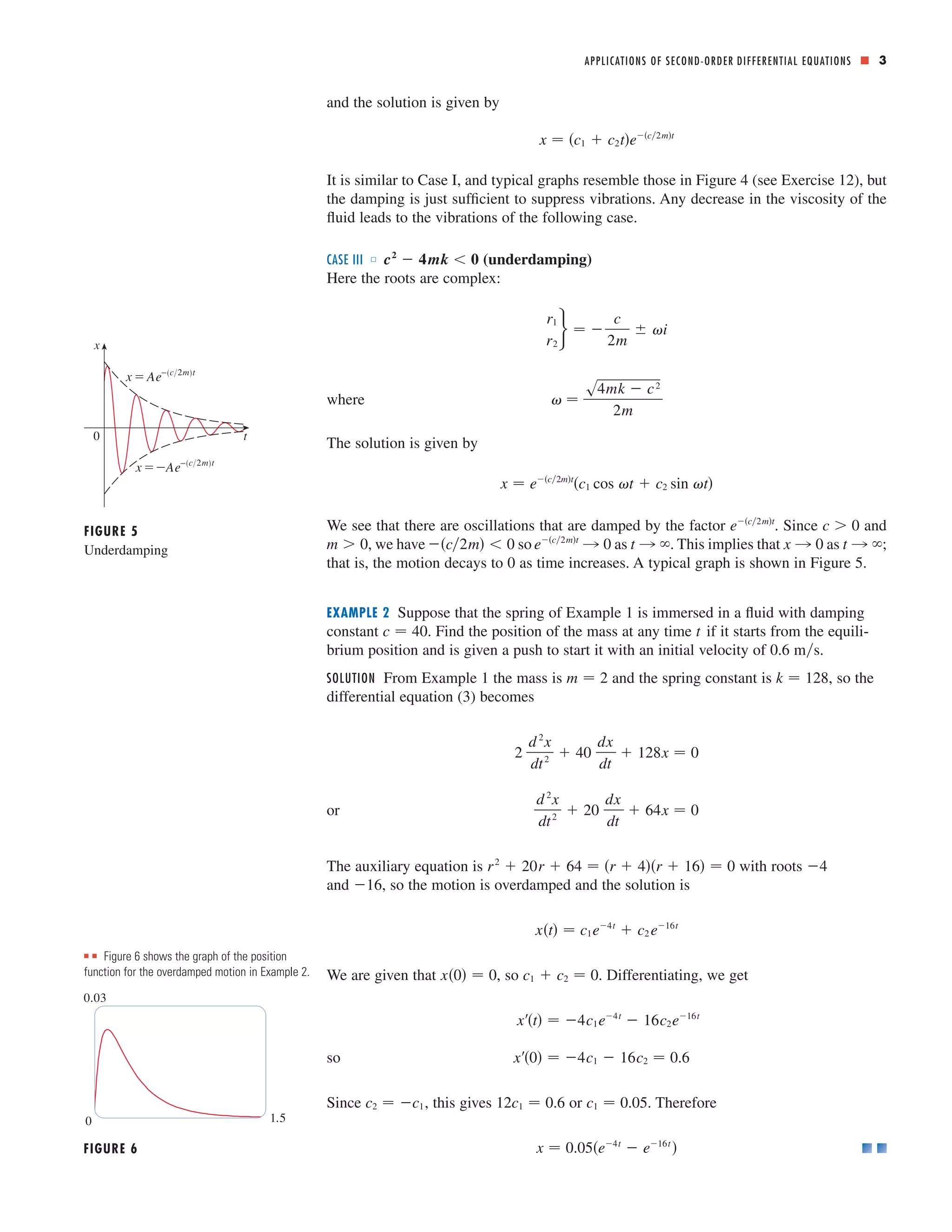
Explains damped motion in springs, includes overdamping, underdamping, and introduces external forces in vibrations.
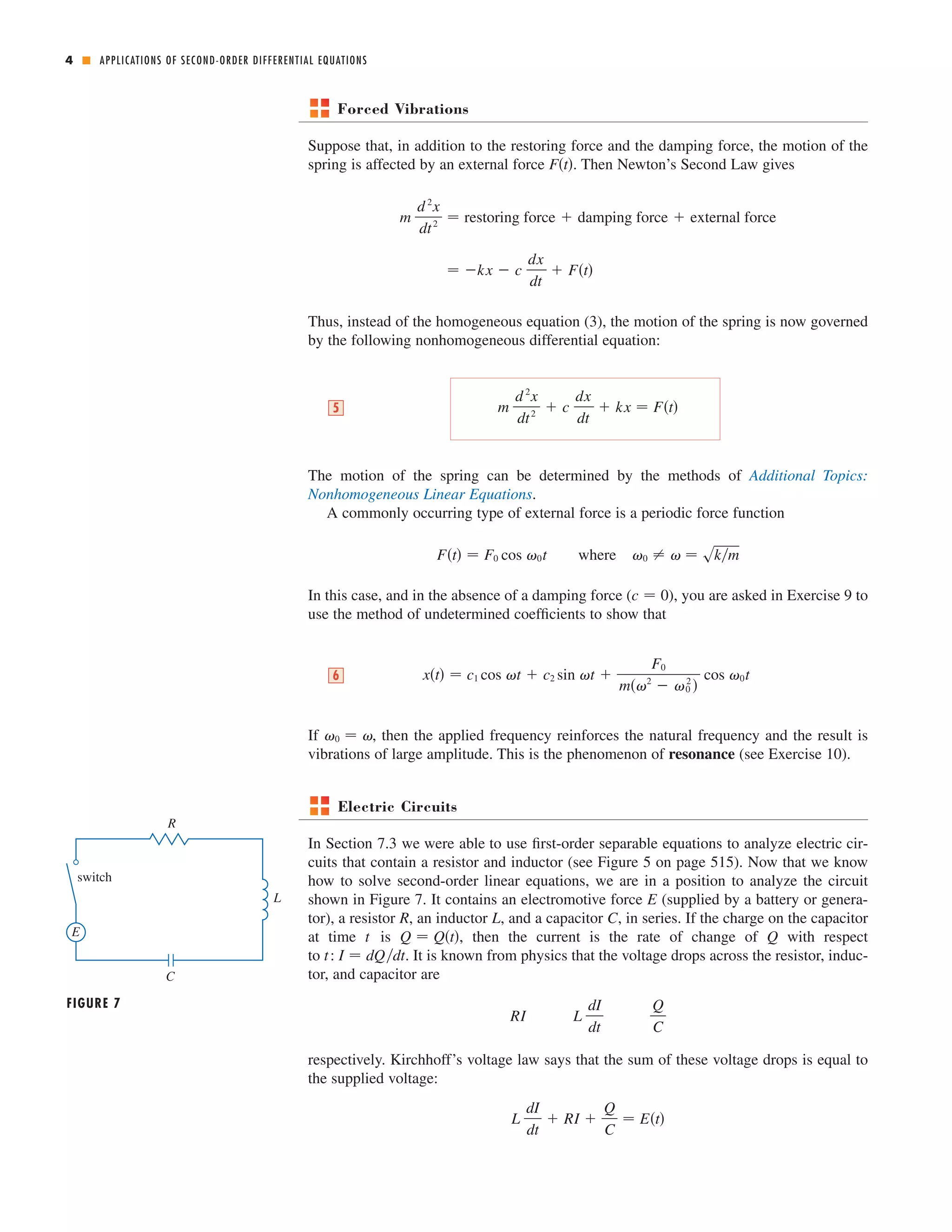
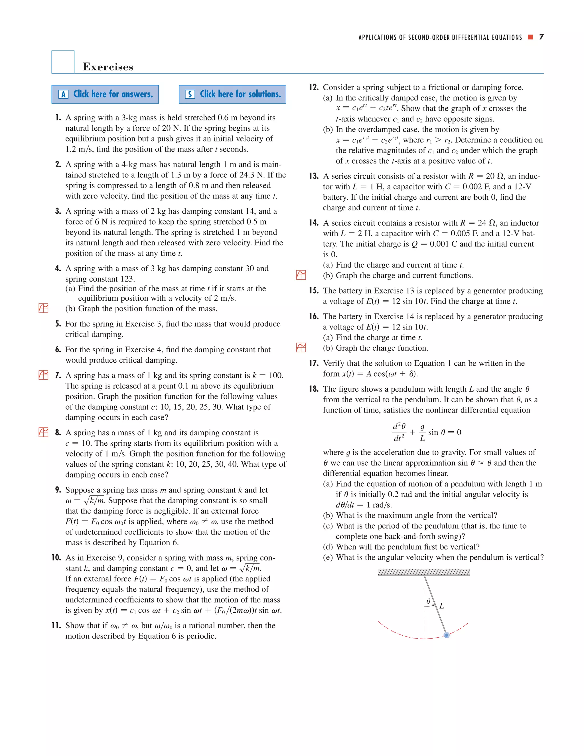
Presents exercises related to spring dynamics and electric circuits, emphasizing critical thinking and application of learned concepts.


![Week 8 [compatibility mode]](https://cdn.slidesharecdn.com/ss_thumbnails/week8compatibilitymode-130213163443-phpapp01-thumbnail.jpg?width=640&height=640&fit=bounds)


