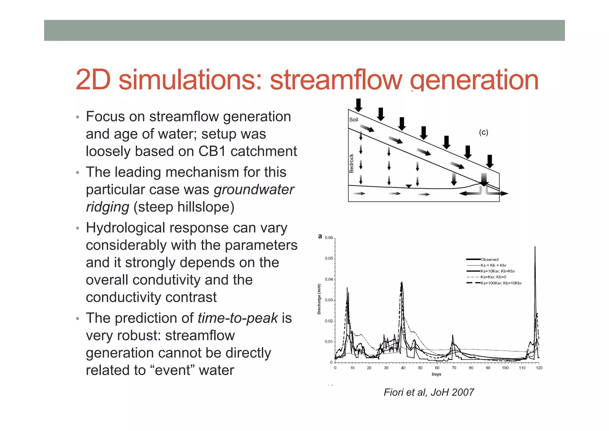
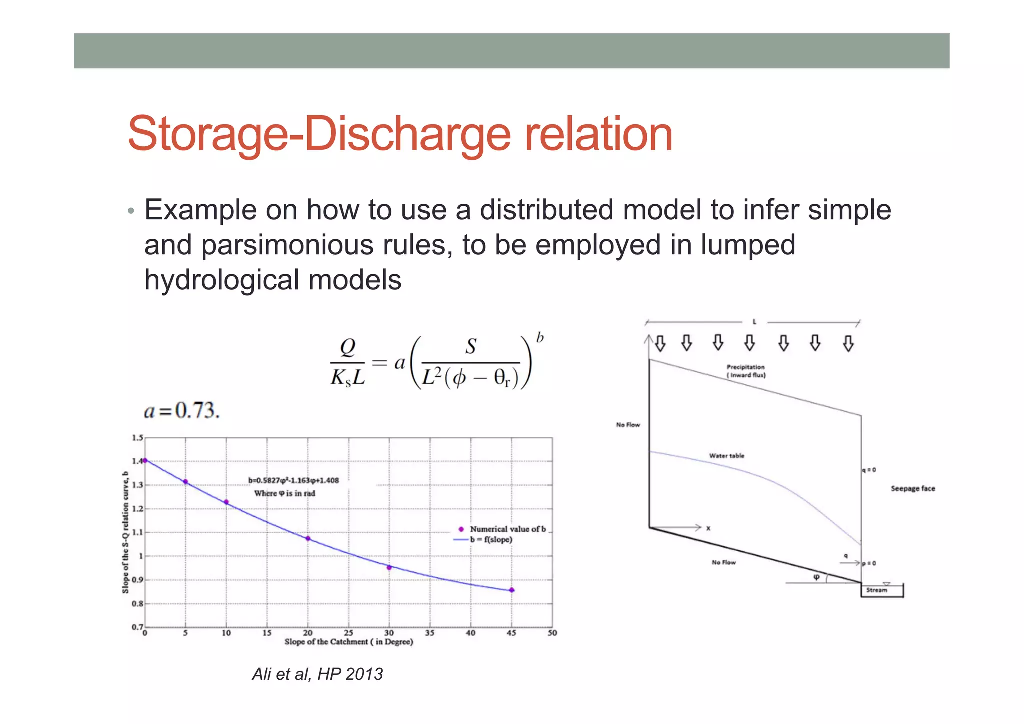
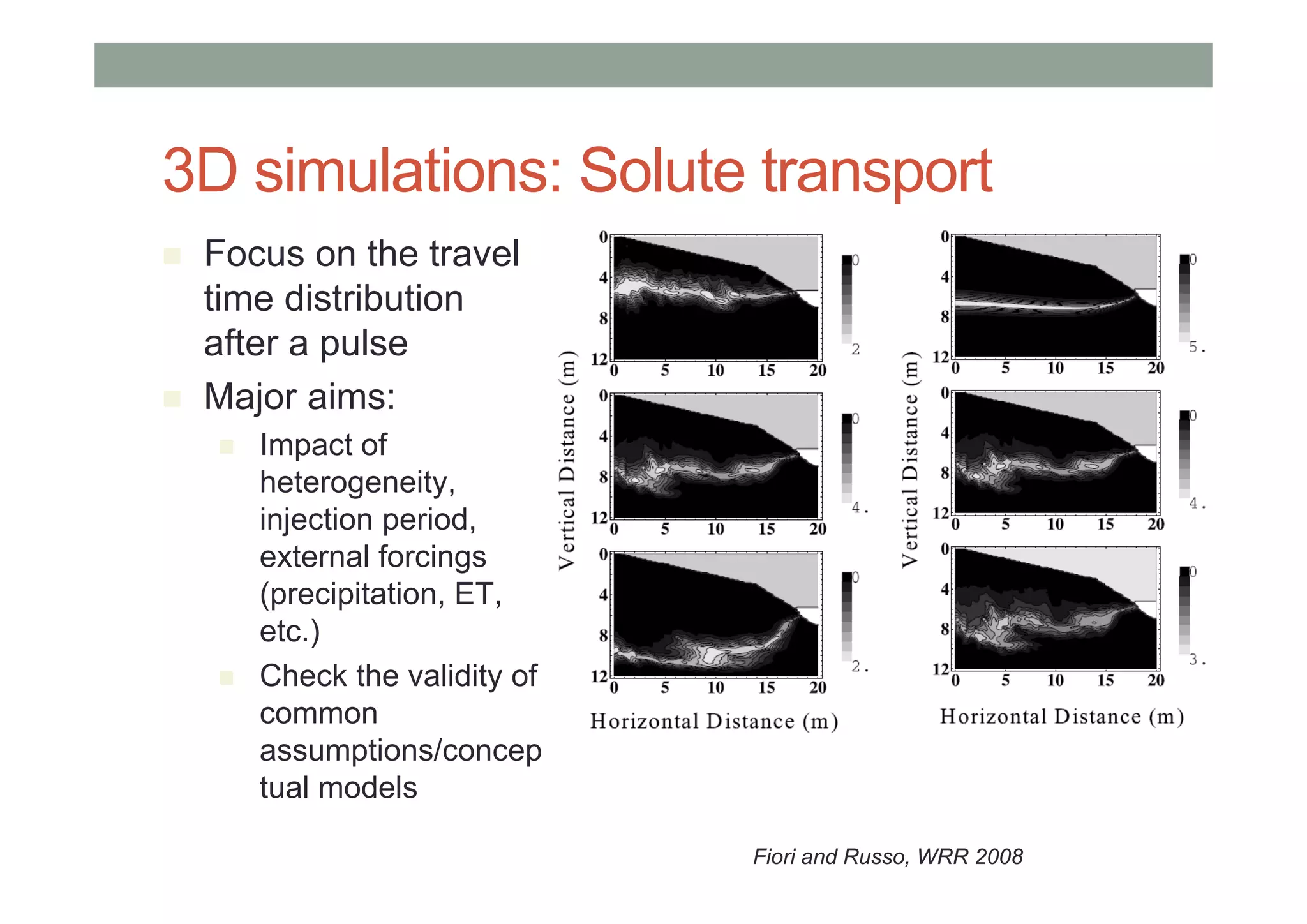
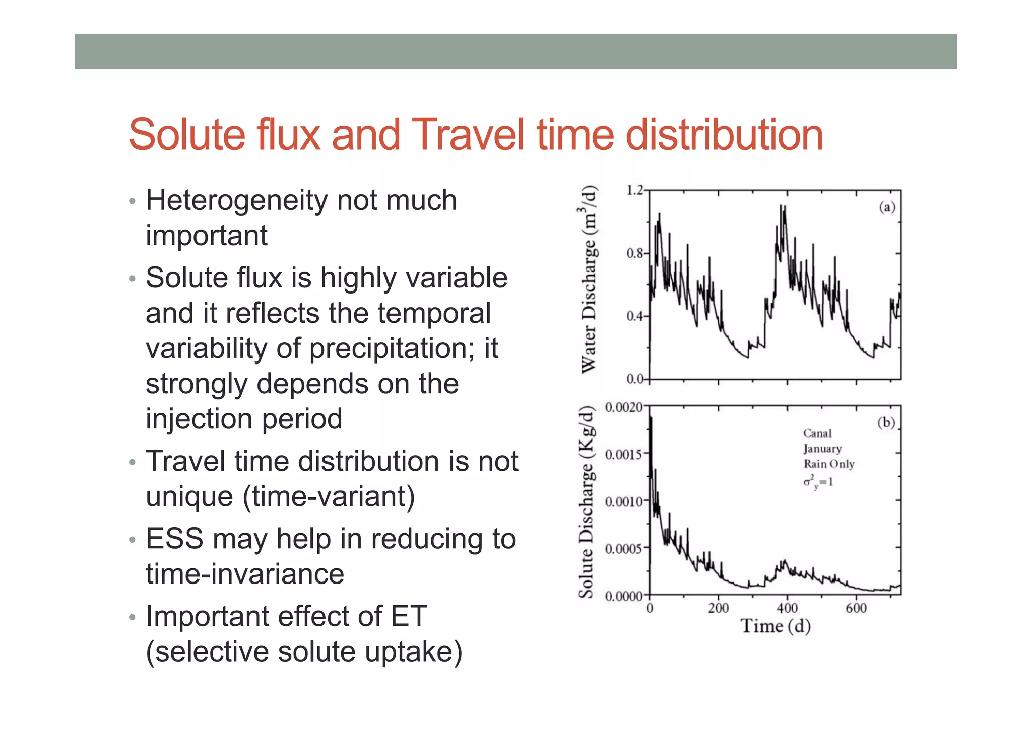
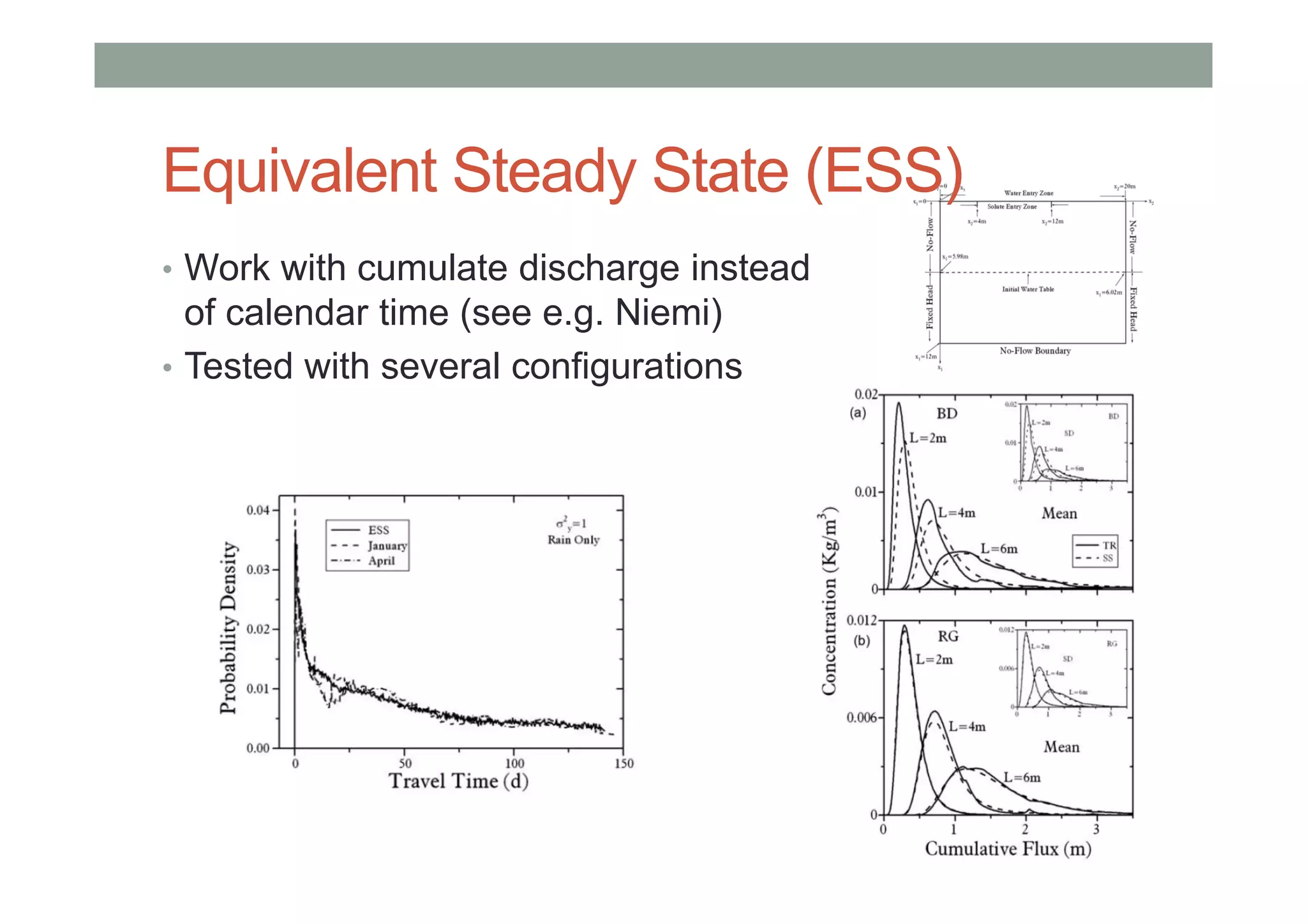
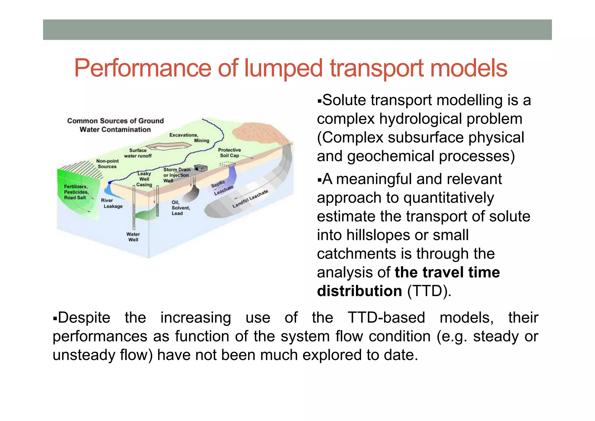
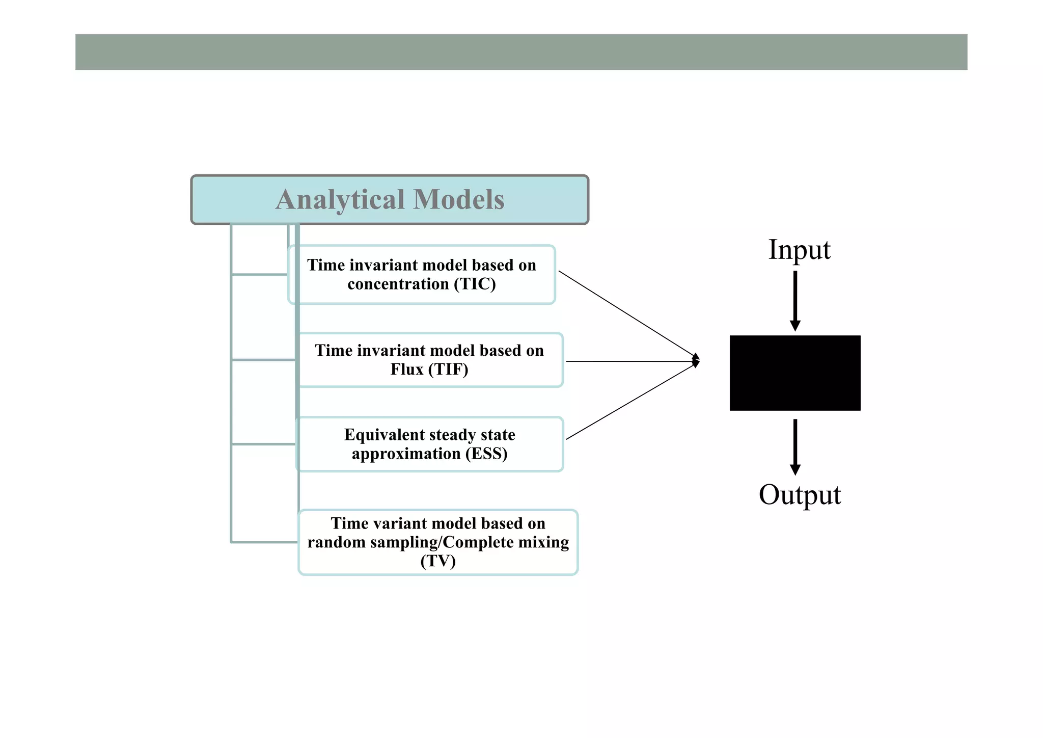
Lessons (I have) learned from
physically-based hydrological models
Aldo Fiori
Università di Roma Tre, Italy
Workshop on coupled hydrological modeling
University of Padova, 23‐24 September 2015.
Role of distributed hydrological models
• Many processes of interest need further
investigation, e.g. streamflow generation
(rainfall-runoff transformation) solute
transport and travel time distribution, SW-
GW interactions, etc.
• Detailed numerical laboratories are useful
tools for understanding: not much/only for
predictions (complexity,
overparametrization, etc.) but as:
• numerical (virtual) experiments for understanding
• help formulate simplified and parsimonious models
• cheking hypotheses and models performance
• Particularly useful for hillslope processes,
that have a central role in catchment
hydrology (limited size, complexity of the
system and processes)
2D simulations: streamflow generation
• Focus on streamflow generation
and age of water; setup was
loosely based on CB1 catchment
• The leading mechanism for this
particular case was groundwater
ridging (steep hillslope)
• Hydrological response can vary
considerably with the parameters
and it strongly depends on the
overall condutivity and the
conductivity contrast
• The prediction of time-to-peak is
very robust: streamflow
generation cannot be directly
related to “event” water
Fiori et al, JoH 2007
2D simulations: Age of water
• Method: Continuous injection of a tracer
• Stream water is mostly “old”
• Partitioning mainly depends on the hillslope geometry and
the soil/bedrock conductivity contrast
Storage-Discharge relation
• Example on how to use a distributed model to infer simple
and parsimonious rules, to be employed in lumped
hydrological models
Ali et al, HP 2013
Insight from simpler models
• Useful information can be obtained through simple
models, less «realistic» but more prone to generalization
(still physically based); Approximations are dictated by
evidence from more complex simulations.
• Boussinesq flow: Dupuit assumption and «complete
mixing» in the vertical.
Fiori, WRR 2012
Complete mixing??
• Complete (or perfect) mixing
seldom encountered, even in the
vertical
• Reformulation of 2D purely-
advective transport and
integration along the vertical
vertical (assuming Dupuit)
• The final ADE is identical to the
one assuming perfect mixing
• Reason: «vertical sampling»
replaces «complete mixing»
• Mixing within the entire system
(reactor) is harder to justify
(relation to StorAGE function)
Courtesy of John Selker
Again on old water contribution..
• The important role of old
water is confirmed
• It is ruled by two simple
dimensionless parameters:
• The ratio between rain water
and pre-event water is crucial
• The dynamic component is not
so important
• The vertically integrated
ADE can be used for more
complex problems involving
advective transport at the
hillslope scale (no mixing is
involved!)
StorAGE functions
• Simple, Boussinesq-like models can be very helpful to gain insight on
the StorAGE selection function through a fully hydrodinamic model
• Example for steady-flow (analytical solution; more work on the way…)
3D simulations: Flow
• 3D, fully
saturated/unsaturated,
heterogeneous setup;
system is ergodic;
Soil+subsoil system with
different properties
• Groundwater ridging is the
leading mechanism
• Hortonian flow is absent;
Direct precipitation on
saturated zone near the
river is present; ponded
areas vary in time
Fiori and Russo, WRR 2007
3D simulations: Solute transport
 Focus on the travel
time distribution
after a pulse
 Major aims:
 Impact of
heterogeneity,
injection period,
external forcings
(precipitation, ET,
etc.)
 Check the validity of
common
assumptions/concep
tual models
Fiori and Russo, WRR 2008
Solute flux and Travel time distribution
• Heterogeneity not much
important
• Solute flux is highly variable
and it reflects the temporal
variability of precipitation; it
strongly depends on the
injection period
• Travel time distribution is not
unique (time-variant)
• ESS may help in reducing to
time-invariance
• Important effect of ET
(selective solute uptake)
Equivalent Steady State (ESS)
• Work with cumulate discharge instead
of calendar time (see e.g. Niemi)
• Tested with several configurations
Why the Gamma distribution?
• Power law: mainly determined
by fast, unsaturated flow in the
upper soil; exponent related to
soil properties;
• Exponential decay:
groundwater contribution
• Heterogeneity not important;
source-zone dispersion
dominates (similar to Rinaldo,
Marani, Rigon, 1991)
• Conclusions different from
Kirchner et al. (2000; 2001)
Solute transport modelling is a
complex hydrological problem
(Complex subsurface physical
and geochemical processes)
A meaningful and relevant
approach to quantitatively
estimate the transport of solute
into hillslopes or small
catchments is through the
analysis of the travel time
distribution (TTD).
Despite the increasing use of the TTD-based models, their
performances as function of the system flow condition (e.g. steady or
unsteady flow) have not been much explored to date.
Performance of lumped transport models
Virtual (numerical) experiments can help evaluate the
performance of some travel-time based models (Time invariant
and time variant).
The models are tested against the results from detailed and
high resolution numerical experiments employing a three
dimensional (3D) dynamic model of a conceptual hillslope with
real hydrological input (i.e. rainfall).
Advantage: all system variables and input/output are perfectly
known
Disadvantage: it’s not a real experiment!
Performance of lumped transport models
Numerical modelling
Flow – Richards Equation
•Transport – Advection – Diffusion
Equation Analytical
Solute
Transport
ModelsData sets
 Rainfall and Evaporation Data
(Denno, northern Italy, which belongs
to the Mediterranean humid climate)
 The hydraulic properties of the
system are heterogeneous, i.e. spatially
distributed – Random space function
Evaluation
Mass recovery
and
Concentration
Performance of lumped transport models
Analytical Models
Time invariant model based on
concentration (TIC)
Time invariant model based on
Flux (TIF)
Equivalent steady state
approximation (ESS)
Time variant model based on
random sampling/Complete mixing
(TV)
Input
Output
Time invariant model
based on concentration
(TIC)
Time invariant model based
on Flux (TIF)
Equivalent steady state
approximation (ESS)
Time variant model based on
random sampling (TV)
A widely employed approach
assuming a time-invariant travel time distribution
strictly valid only when the subsurface flow is stationary
Does not generally fulfil the basic continuity mass requirement under unsteady
flow conditions
where C₀(t) is inflow concentration, C(t) is the cumulated
outflow volume ps(t) is the transit time distribution (i.e. gamma)



0
00 )()()(*)()(  dtpCtptCtC ss
Replaced solute concentration with mass flux in the convolution in TIC model
Always fulfills mass continuity, and the total mass is recovered from the system
Partition parameter is introduced in order to model in the presence of
evapotranspiration (Botter et al.,2010)
 Thus, the solute fluxes which exit the system through Q and ET are written as
Time invariant model based
on concentration (TIC)
Time invariant model
based on Flux (TIF)
Equivalent steady state
approximation (ESS)
Time variant model based on
random sampling (TV)
where Q₀(t) is inflow, Q(t) is the cumulated outflow volume
ET(t) is evapotranspiration
       


0
0  dtpFtF sQ
        


0
0 1  dtpFtF ETET
)()()( 000 tCtQtF 
)()()( tCtQtF QQ 
Time invariant model based
on concentration (TIC)
Time invariant model based
on Flux (TIF)
Equivalent steady
state approximation
(ESS)
Time variant model based on
random sampling (TV)
ESS model implies that the same convolution appearing in TIC
can be applied by a simple rescaling of calendar times.
(Niemi,1977)
It fully preserves mass continuity
Following the ESS approach, the injection time (τ) and exit
time (t) of the solute flux are expressed by the newly introduced
rescaled times as:
where V₀(t) is the cumulated rainfall volume injected to the
control volume and V(t) is the cumulated outflow volume
     
t
R dQ
QQ
tV
0
0
0 1

   
t
R dQ
QQ
tV
t
0
1

         


0
00 * RRRRRsRRQ tptCdtpCtC 
Time invariant model based
on concentration (TIC)
Time invariant model based
on Flux (TIF)
Equivalent steady state
approximation (ESS) Time variant model based
on random sampling (TV)
It is based on a time-variant formulation of TTD
A more consistent and robust approach to model solute transport
complete and instantaneous mixing between the injected solute
and the water stored in the system is often assumed
Requires the definition of travel time distributions conditioned at
both injection and exit times
where S(t) is the total water storage and M(t) is the total mass in the
system
       tETtQtQ
dt
tdS
 0
       tFtFtF
dt
tdM
ETQ  0
      tCtC
tS
tQ
dt
tdC
 0
0
)(
)(
     
 
 



t dx
xS
xQ
de
S
Q
CtC
t
0
)(0
0
0



 
     
 
 




t dx
xS
xETxQ
de
tS
Q
CtC
t
0
)(
)(
0
0 

 
Calibration is made in the first period (spring) injection,
while validation is performed over the other three periods
(summer, fall, winter)
Two scenarios are considered
•Rain only (RO) in which no ET is present
•Rain and ET case in which ET is considered
In the RET scenario, The partition parameter θ is
calibrated through two step iteration. Three parameter (θ ,β
and α) calibration with constant θ and then assuming the
water flow route is described by the same TTD, temporarilly
variable θ(t) can be obtained through
       dtQtp
tQ
t   ,
)(
1
0
Result and Discussion –numerical
results of study cases
TIC
Result : Raifall only scenario (RO)
Spring
Winter
Injectiontime
TIF
Result : Raifall only scenario (RO)
Spring
Winter
Injectiontime
Result : Raifall only scenario (RO)
ESS
Spring
Winter
Injectiontime
R2 = 0.828
Result : Raifall only scenario (RO)
TV
Spring
Winter
Injectiontime
Comment: zero parameters, but «active» storage needed to be fixed…
Rainfall and ET scenario (RET)
In some of the previous studies, the ET-related solute flux has
been neglected or taken as proportional to the streamflow
concentration (Rodhe et al.,1996; Benettin et al.,2013; Bertuzzo
et al.,2013).
 In fact, solute concentration through the plant roots is typically
much more difficult to measure than concentration streamflow
(Rodhe et al.,1996).
•The relatively poor behavior of all models highlights the
importance of ET when studying solute transport in areas in
which ET is relevant (Van der Velde et al HP2015)
•The total mass is fully recovered. However, only the total mass
is preserved, while the separate contributions MQ and MET may
different from the "real" ones
TV
Result: Raifall and ET scenario (RET)
Spring
Winter
Injectiontime
Conclusions
• Water flow and solute transport in hillslopes are
challenging areas of research
• Role of numerical models:
• Understanding of the principal physical processes
• Test common assumptions/models
• Help in developing and testing simplified models
• Much insight can be gained from models
• Numerical models should be as much realistic as
possible (3D, sat/unsat, SW/GW, uptake by roots,
heterogeneous, etc.)
• Simple, lumped models are necessary, but they need to
have strong physical foundations
References
• Ali, M., A. Fiori, G. Bellotti, Analysis of the nonlinear storage-discharge relation for hillslope
through 2D numerical modelling. HYDROLOGICAL PROCESSES, 27:2683-2690, DOI:
10.1002/hyp.9397, 2013
• Ali, M., A. Fiori, D. Russo, A comparison of travel-time based catchment transport models, with
application to numerical experiments, JOURNAL OF HYDROLOGY, 511, pg. 605-
618, http://dx.doi.org/10.1016/j.jhydrol.2014.02.010, 2014.
• Fiori, A. Old water contribution to streamflow: Insight from a linear Boussinesq model. WATER
RESOURCES RESEARCH, 48(6), W06601, DOI: 10.1029/2011WR011606, 2012
• Fiori, A., M. Romanelli, D.J. Cavalli, D.Russo, Numerical experiments of streamflow generation in
steep catchments, JOURNAL OF HYDROLOGY, 339, 183-192, 2007.
• Fiori, A., D. Russo, Numerical Analyses of Subsurface Flow in a Steep Hillslope under Rainfall:
The Role of the Spatial Heterogeneity of the Formation Hydraulic Properties, WATER RESOURCES
RESEARCH, 43, W07445, doi:10.1029/2006WR005365, 2007
• Russo, D., A. Fiori. Equivalent Vadose Zone Steady-State Flow: An Assessment of its Capability
to Predict Transport in a Realistic Combined Vadose Zone - Groundwater Flow System. WATER
RESOURCES RESEARCH, 44, W09436, doi:10.1029/ 2007WR006170, 2008.
• Fiori, A., D. Russo, Travel Time Distribution in a Hillslope: Insight from Numerical Simulations.
WATER RESOURCES RESEARCH, 44, W12426, doi:10.1029/2008WR007135, 2008.
• Russo, D., and A. Fiori, Stochastic analysis of transport in a combined heterogeneous vadose
zone–groundwater flow system. WATER RESOURCES RESEARCH, 45, W03426,
doi:10.1029/2008WR007157, 2009.
• Fiori, A., D. Russo, M. Di Lazzaro. Stochastic analysis of transport in hillslopes: Travel time
distribution and source zone dispersion. WATER RESOURCES RESEARCH, 45, W08435, 2009.

Aldo Fiori

  • 1.
    Lessons (I have)learned from physically-based hydrological models Aldo Fiori Università di Roma Tre, Italy Workshop on coupled hydrological modeling University of Padova, 23‐24 September 2015.
  • 2.
    Role of distributedhydrological models • Many processes of interest need further investigation, e.g. streamflow generation (rainfall-runoff transformation) solute transport and travel time distribution, SW- GW interactions, etc. • Detailed numerical laboratories are useful tools for understanding: not much/only for predictions (complexity, overparametrization, etc.) but as: • numerical (virtual) experiments for understanding • help formulate simplified and parsimonious models • cheking hypotheses and models performance • Particularly useful for hillslope processes, that have a central role in catchment hydrology (limited size, complexity of the system and processes)
  • 3.
    2D simulations: streamflowgeneration • Focus on streamflow generation and age of water; setup was loosely based on CB1 catchment • The leading mechanism for this particular case was groundwater ridging (steep hillslope) • Hydrological response can vary considerably with the parameters and it strongly depends on the overall condutivity and the conductivity contrast • The prediction of time-to-peak is very robust: streamflow generation cannot be directly related to “event” water Fiori et al, JoH 2007
  • 4.
    2D simulations: Ageof water • Method: Continuous injection of a tracer • Stream water is mostly “old” • Partitioning mainly depends on the hillslope geometry and the soil/bedrock conductivity contrast
  • 5.
    Storage-Discharge relation • Exampleon how to use a distributed model to infer simple and parsimonious rules, to be employed in lumped hydrological models Ali et al, HP 2013
  • 6.
    Insight from simplermodels • Useful information can be obtained through simple models, less «realistic» but more prone to generalization (still physically based); Approximations are dictated by evidence from more complex simulations. • Boussinesq flow: Dupuit assumption and «complete mixing» in the vertical. Fiori, WRR 2012
  • 7.
    Complete mixing?? • Complete(or perfect) mixing seldom encountered, even in the vertical • Reformulation of 2D purely- advective transport and integration along the vertical vertical (assuming Dupuit) • The final ADE is identical to the one assuming perfect mixing • Reason: «vertical sampling» replaces «complete mixing» • Mixing within the entire system (reactor) is harder to justify (relation to StorAGE function) Courtesy of John Selker
  • 8.
    Again on oldwater contribution.. • The important role of old water is confirmed • It is ruled by two simple dimensionless parameters: • The ratio between rain water and pre-event water is crucial • The dynamic component is not so important • The vertically integrated ADE can be used for more complex problems involving advective transport at the hillslope scale (no mixing is involved!)
  • 9.
    StorAGE functions • Simple,Boussinesq-like models can be very helpful to gain insight on the StorAGE selection function through a fully hydrodinamic model • Example for steady-flow (analytical solution; more work on the way…)
  • 10.
    3D simulations: Flow •3D, fully saturated/unsaturated, heterogeneous setup; system is ergodic; Soil+subsoil system with different properties • Groundwater ridging is the leading mechanism • Hortonian flow is absent; Direct precipitation on saturated zone near the river is present; ponded areas vary in time Fiori and Russo, WRR 2007
  • 11.
    3D simulations: Solutetransport  Focus on the travel time distribution after a pulse  Major aims:  Impact of heterogeneity, injection period, external forcings (precipitation, ET, etc.)  Check the validity of common assumptions/concep tual models Fiori and Russo, WRR 2008
  • 12.
    Solute flux andTravel time distribution • Heterogeneity not much important • Solute flux is highly variable and it reflects the temporal variability of precipitation; it strongly depends on the injection period • Travel time distribution is not unique (time-variant) • ESS may help in reducing to time-invariance • Important effect of ET (selective solute uptake)
  • 13.
    Equivalent Steady State(ESS) • Work with cumulate discharge instead of calendar time (see e.g. Niemi) • Tested with several configurations
  • 14.
    Why the Gammadistribution? • Power law: mainly determined by fast, unsaturated flow in the upper soil; exponent related to soil properties; • Exponential decay: groundwater contribution • Heterogeneity not important; source-zone dispersion dominates (similar to Rinaldo, Marani, Rigon, 1991) • Conclusions different from Kirchner et al. (2000; 2001)
  • 15.
    Solute transport modellingis a complex hydrological problem (Complex subsurface physical and geochemical processes) A meaningful and relevant approach to quantitatively estimate the transport of solute into hillslopes or small catchments is through the analysis of the travel time distribution (TTD). Despite the increasing use of the TTD-based models, their performances as function of the system flow condition (e.g. steady or unsteady flow) have not been much explored to date. Performance of lumped transport models
  • 16.
    Virtual (numerical) experimentscan help evaluate the performance of some travel-time based models (Time invariant and time variant). The models are tested against the results from detailed and high resolution numerical experiments employing a three dimensional (3D) dynamic model of a conceptual hillslope with real hydrological input (i.e. rainfall). Advantage: all system variables and input/output are perfectly known Disadvantage: it’s not a real experiment! Performance of lumped transport models
  • 17.
    Numerical modelling Flow –Richards Equation •Transport – Advection – Diffusion Equation Analytical Solute Transport ModelsData sets  Rainfall and Evaporation Data (Denno, northern Italy, which belongs to the Mediterranean humid climate)  The hydraulic properties of the system are heterogeneous, i.e. spatially distributed – Random space function Evaluation Mass recovery and Concentration Performance of lumped transport models
  • 18.
    Analytical Models Time invariantmodel based on concentration (TIC) Time invariant model based on Flux (TIF) Equivalent steady state approximation (ESS) Time variant model based on random sampling/Complete mixing (TV) Input Output
  • 19.
    Time invariant model basedon concentration (TIC) Time invariant model based on Flux (TIF) Equivalent steady state approximation (ESS) Time variant model based on random sampling (TV) A widely employed approach assuming a time-invariant travel time distribution strictly valid only when the subsurface flow is stationary Does not generally fulfil the basic continuity mass requirement under unsteady flow conditions where C₀(t) is inflow concentration, C(t) is the cumulated outflow volume ps(t) is the transit time distribution (i.e. gamma)    0 00 )()()(*)()(  dtpCtptCtC ss
  • 20.
    Replaced solute concentrationwith mass flux in the convolution in TIC model Always fulfills mass continuity, and the total mass is recovered from the system Partition parameter is introduced in order to model in the presence of evapotranspiration (Botter et al.,2010)  Thus, the solute fluxes which exit the system through Q and ET are written as Time invariant model based on concentration (TIC) Time invariant model based on Flux (TIF) Equivalent steady state approximation (ESS) Time variant model based on random sampling (TV) where Q₀(t) is inflow, Q(t) is the cumulated outflow volume ET(t) is evapotranspiration           0 0  dtpFtF sQ            0 0 1  dtpFtF ETET )()()( 000 tCtQtF  )()()( tCtQtF QQ 
  • 21.
    Time invariant modelbased on concentration (TIC) Time invariant model based on Flux (TIF) Equivalent steady state approximation (ESS) Time variant model based on random sampling (TV) ESS model implies that the same convolution appearing in TIC can be applied by a simple rescaling of calendar times. (Niemi,1977) It fully preserves mass continuity Following the ESS approach, the injection time (τ) and exit time (t) of the solute flux are expressed by the newly introduced rescaled times as: where V₀(t) is the cumulated rainfall volume injected to the control volume and V(t) is the cumulated outflow volume       t R dQ QQ tV 0 0 0 1      t R dQ QQ tV t 0 1              0 00 * RRRRRsRRQ tptCdtpCtC 
  • 22.
    Time invariant modelbased on concentration (TIC) Time invariant model based on Flux (TIF) Equivalent steady state approximation (ESS) Time variant model based on random sampling (TV) It is based on a time-variant formulation of TTD A more consistent and robust approach to model solute transport complete and instantaneous mixing between the injected solute and the water stored in the system is often assumed Requires the definition of travel time distributions conditioned at both injection and exit times where S(t) is the total water storage and M(t) is the total mass in the system        tETtQtQ dt tdS  0        tFtFtF dt tdM ETQ  0       tCtC tS tQ dt tdC  0 0 )( )(              t dx xS xQ de S Q CtC t 0 )(0 0 0                    t dx xS xETxQ de tS Q CtC t 0 )( )( 0 0    
  • 23.
    Calibration is madein the first period (spring) injection, while validation is performed over the other three periods (summer, fall, winter) Two scenarios are considered •Rain only (RO) in which no ET is present •Rain and ET case in which ET is considered In the RET scenario, The partition parameter θ is calibrated through two step iteration. Three parameter (θ ,β and α) calibration with constant θ and then assuming the water flow route is described by the same TTD, temporarilly variable θ(t) can be obtained through        dtQtp tQ t   , )( 1 0
  • 24.
    Result and Discussion–numerical results of study cases
  • 25.
    TIC Result : Raifallonly scenario (RO) Spring Winter Injectiontime
  • 26.
    TIF Result : Raifallonly scenario (RO) Spring Winter Injectiontime
  • 27.
    Result : Raifallonly scenario (RO) ESS Spring Winter Injectiontime R2 = 0.828
  • 28.
    Result : Raifallonly scenario (RO) TV Spring Winter Injectiontime Comment: zero parameters, but «active» storage needed to be fixed…
  • 29.
    Rainfall and ETscenario (RET) In some of the previous studies, the ET-related solute flux has been neglected or taken as proportional to the streamflow concentration (Rodhe et al.,1996; Benettin et al.,2013; Bertuzzo et al.,2013).  In fact, solute concentration through the plant roots is typically much more difficult to measure than concentration streamflow (Rodhe et al.,1996). •The relatively poor behavior of all models highlights the importance of ET when studying solute transport in areas in which ET is relevant (Van der Velde et al HP2015) •The total mass is fully recovered. However, only the total mass is preserved, while the separate contributions MQ and MET may different from the "real" ones
  • 30.
    TV Result: Raifall andET scenario (RET) Spring Winter Injectiontime
  • 31.
    Conclusions • Water flowand solute transport in hillslopes are challenging areas of research • Role of numerical models: • Understanding of the principal physical processes • Test common assumptions/models • Help in developing and testing simplified models • Much insight can be gained from models • Numerical models should be as much realistic as possible (3D, sat/unsat, SW/GW, uptake by roots, heterogeneous, etc.) • Simple, lumped models are necessary, but they need to have strong physical foundations
  • 32.
    References • Ali, M.,A. Fiori, G. Bellotti, Analysis of the nonlinear storage-discharge relation for hillslope through 2D numerical modelling. HYDROLOGICAL PROCESSES, 27:2683-2690, DOI: 10.1002/hyp.9397, 2013 • Ali, M., A. Fiori, D. Russo, A comparison of travel-time based catchment transport models, with application to numerical experiments, JOURNAL OF HYDROLOGY, 511, pg. 605- 618, http://dx.doi.org/10.1016/j.jhydrol.2014.02.010, 2014. • Fiori, A. Old water contribution to streamflow: Insight from a linear Boussinesq model. WATER RESOURCES RESEARCH, 48(6), W06601, DOI: 10.1029/2011WR011606, 2012 • Fiori, A., M. Romanelli, D.J. Cavalli, D.Russo, Numerical experiments of streamflow generation in steep catchments, JOURNAL OF HYDROLOGY, 339, 183-192, 2007. • Fiori, A., D. Russo, Numerical Analyses of Subsurface Flow in a Steep Hillslope under Rainfall: The Role of the Spatial Heterogeneity of the Formation Hydraulic Properties, WATER RESOURCES RESEARCH, 43, W07445, doi:10.1029/2006WR005365, 2007 • Russo, D., A. Fiori. Equivalent Vadose Zone Steady-State Flow: An Assessment of its Capability to Predict Transport in a Realistic Combined Vadose Zone - Groundwater Flow System. WATER RESOURCES RESEARCH, 44, W09436, doi:10.1029/ 2007WR006170, 2008. • Fiori, A., D. Russo, Travel Time Distribution in a Hillslope: Insight from Numerical Simulations. WATER RESOURCES RESEARCH, 44, W12426, doi:10.1029/2008WR007135, 2008. • Russo, D., and A. Fiori, Stochastic analysis of transport in a combined heterogeneous vadose zone–groundwater flow system. WATER RESOURCES RESEARCH, 45, W03426, doi:10.1029/2008WR007157, 2009. • Fiori, A., D. Russo, M. Di Lazzaro. Stochastic analysis of transport in hillslopes: Travel time distribution and source zone dispersion. WATER RESOURCES RESEARCH, 45, W08435, 2009.