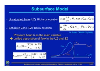
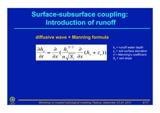
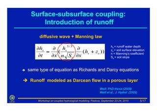
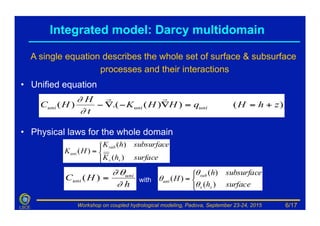
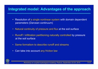
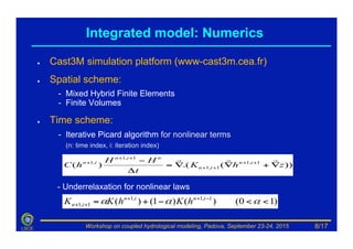
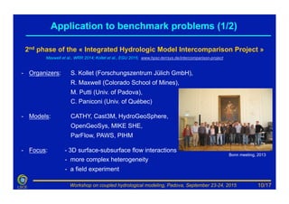
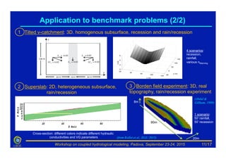
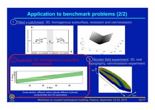
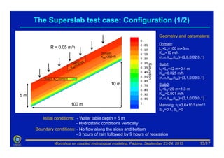
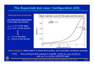
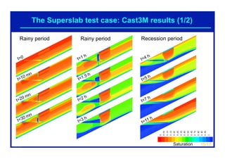
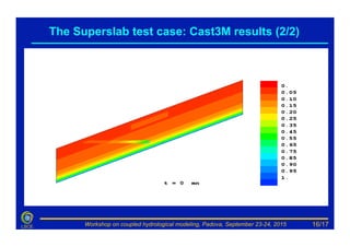
Workshop on coupled hydrological modeling, Padova, September 23-24, 2015LSCE
Darcy multi-domain approach for
coupling surface-subsurface flows:
Application to benchmark problems
Claude MUGLER, Emmanuel MOUCHE
Laboratoire des Sciences du Climat et de l’Environnement
UMR 8212 CEA/CNRS/UVSQ, Orme des Merisiers,
91191 Gif-sur-Yvette, France
1/17
Workshop on coupled hydrological modeling, Padova, September 23-24, 2015LSCE
Summary
•  The integrated model: Description and validation
•  Integrated Hydrologic Model Intercomparison
•  Conclusion
2/17
Workshop on coupled hydrological modeling, Padova, September 23-24, 2015LSCE
–  Unsaturated Zone (UZ): Richards equation
–  Saturated Zone (SZ): Darcy equation
Pressure head h as the main variable
è unified description of flow in the UZ and SZ
)))((.()( zhhK
t
h
hC ∇+∇∇=
!!!
∂
∂
))(.( zhK
t
h
S sat ∇+∇∇=
!!!
∂
∂
⎩
⎨
⎧
=
∂
∂
=
SZinS
UZinhC
h
hC sub
sub
)(
)(
θ
h0
Ksub(h)
Csub(h)
⎩
⎨
⎧
=
SZinK
UZinhK
hK
sat
sub
)(
)(
Ksat
K(h)
C(h)
S
Subsurface Model
Le Potier, CMWR XII (1998)
3/17
Workshop on coupled hydrological modeling, Padova, September 23-24, 2015LSCE
diffusive wave + Manning formula
))((
3/5
ss
s
ss
zh
xSn
h
xt
h
+
∂
∂
∂
∂
=
∂
∂ hs = runoff water depth
zs = soil surface elevation
n = Manning’s coefficient
Ss = soil slope
Surface-subsurface coupling:
Introduction of runoff
4/17
Workshop on coupled hydrological modeling, Padova, September 23-24, 2015LSCE
diffusive wave + Manning law
))((
3/5
ss
s
ss
zh
xSn
h
xt
h
+
∂
∂
∂
∂
=
∂
∂ hs = runoff water depth
zs = soil surface elevation
n = Manning’s coefficient
Ss = soil slope
Surface-subsurface coupling:
Introduction of runoff
5/17
è  same type of equation as Richards and Darcy equations
è  Runoff modeled as Darcean flow in a porous layer
Weill, PhD thesis (2008)
Weill et al., J. Hydrol. (2009)
Workshop on coupled hydrological modeling, Padova, September 23-24, 2015LSCE
•  Unified equation
)())(.()( zhHqHHK
t
H
HC uniuniuni +==∇−∇−
!!
∂
∂
Integrated model: Darcy multidomain
•  Physical laws for the whole domain
⎪⎩
⎪
⎨
⎧
=
surfacehK
subsurfacehK
HK
ss
sub
uni
)(
)(
)(
⎩
⎨
⎧
=
surfaceh
subsurfaceh
H
ss
sub
uni
)(
)(
)(
θ
θ
θ
h
HC uni
uni
∂
θ∂
=)( with
A single equation describes the whole set of surface & subsurface
processes and their interactions
6/17
Workshop on coupled hydrological modeling, Padova, September 23-24, 2015LSCE
•  Resolution of a single nonlinear system with domain dependent
parameters (Darcean continuum)
•  Natural continuity of pressure and flux at the soil surface
•  Runoff / infiltration partitioning naturally controlled by pressure
at the soil surface
•  Same formalism to describe runoff and streams
•  Can take into account any friction law
Integrated model: Advantages of the approach
7/17
Workshop on coupled hydrological modeling, Padova, September 23-24, 2015LSCE
●  Cast3M simulation platform (www-cast3m.cea.fr)
●  Spatial scheme:
- Mixed Hybrid Finite Elements
- Finite Volumes
●  Time scheme:
- Iterative Picard algorithm for nonlinear terms
(n: time index, i: iteration index)
- Underrelaxation for nonlinear laws
))(.()( 1,1
1,1
1,1
,1
zhK
t
HH
hC in
in
nin
in
∇+∇∇=
Δ
− ++
++
++
+
!!!
)10()()1()( 1,1,1
1,1 <<−+= −++
++ ααα inin
in hKhKK
Integrated model: Numerics
8/17
Workshop on coupled hydrological modeling, Padova, September 23-24, 2015LSCE
Abdul and Gillham (WRR, 1984)
Ogden and Watts (WRR, 2000)Govindaraju and Kavvas (WRR, 1991)
Di Giammarco et al (J Hydrol 1996)
Mugler et al ( sub. J Hydrol)
Vauclin et al (WRR, 1978)
Subsurface flow and transport
Overland flow model
Integrated surface/subsurface model
outlet
saturated zone
unsaturated
zone
Rainfall
prescribed head boundary
no flow boundaries
saturated length
3D configuration
Validation & Application
9/17
Weill, PhD thesis (2008); Weill et al., J. Hydrol. (2009)
Workshop on coupled hydrological modeling, Padova, September 23-24, 2015LSCE
2nd phase of the « Integrated Hydrologic Model Intercomparison Project »
Maxwell et al., WRR 2014; Kollet et al., EGU 2015; www.hpsc-terrsys.de/intercomparison-project
-  Organizers: S. Kollet (Forschungszentrum Jülich GmbH),
R. Maxwell (Colorado School of Mines),
M. Putti (Univ. of Padova),
C. Paniconi (Univ. of Québec)
-  Models: CATHY, Cast3M, HydroGeoSphere,
OpenGeoSys, MIKE SHE,
ParFlow, PAWS, PIHM
-  Focus: - 3D surface-subsurface flow interactions
- more complex heterogeneity
- a field experiment
Bonn meeting, 2013
Application to benchmark problems (1/2)
10/17
Workshop on coupled hydrological modeling, Padova, September 23-24, 2015LSCE
1 Tilted v-catchment: 3D, homogenous subsurface, recession and rain/recession
3 Borden field experiment: 3D, real
topography, rain/recession experiment
2 Superslab: 2D, heterogeneous subsurface,
rain/recession
Application to benchmark problems (2/2)
Cross-section: different colors indicate different hydraulic
conductivities and VG parameters
80m
20m
8m
80m
(from Kollet et al., EGU 2015)
11/17
(Abdul &
Gillham, 1989)
4 scenarios:
recession,
rainfall,
various nManning
1 scenario:
50’ rainfall,
50’ recession
Workshop on coupled hydrological modeling, Padova, September 23-24, 2015LSCE
1 Tilted v-catchment: 3D, homogenous subsurface, recession and rain/recession
3 Borden field experiment: 3D, real
topography, rain/recession experiment
2 Superslab: 2D, heterogeneous subsurface,
rain/recession
Application to benchmark problems (2/2)
Cross-section: different colors indicate different hydraulic
conductivities and VG parameters
80m
20m
8m
12/17
Workshop on coupled hydrological modeling, Padova, September 23-24, 2015LSCE
The Superslab test case: Configuration (1/2)
Geometry and parameters:
Domain:
Lx×Lz=100 m×5 m
Ksat=10 m/h
(n,α,θres,θsat)=(2,6,0.02,0.1)
Slab1:
Lx×Lz=42 m×0.4 m
Ksat=0.025 m/h
(n,α,θres,θsat)=(3,1,0.03,0.1)
Slab2:
Lx×Lz=20 m×1.3 m
Ksat=0.001 m/h
(n,α,θres,θsat)=(3,1,0.03,0.1)
Manning: nc=3.6×10⁻³ s/m1/3
Sf,x=0.1, Sf,z=0
13/17
Domain:
Ksat=200×R
R = 0.05 m/h
Slab1: Ksat=0.5×R
100 m
5 m
10 m
Saturation
Initial conditions: - Water table depth = 5 m
- Hydrostatic conditions vertically
Boundary conditions: - No flow along the sides and bottom
- 3 hours of rain followed by 9 hours of recession
Workshop on coupled hydrological modeling, Padova, September 23-24, 2015LSCE
Initial conditions: Water table 5 m below land surface, and hydrostatic conditions vertically
The Superslab test case: Configuration (2/2)
14/17
Heterogeneous properties:
1 m
20 cm
Very small grid cells required in Cast3M: 5×10⁻⁵ m < Δz < 5×10⁻² m
with Δx=1 m, Nx×Nz=100×2015 cells
αVG = 1 m-1 in the slabs
αVG = 6 m-1 in the domain
Lc ~ 1 m in the slabs
Lc ~ 20 cm in the domain
van Genuchten parameters
in the slabs and domain:
Water retention curve for the slabs and the domain
Workshop on coupled hydrological modeling, Padova, September 23-24, 2015LSCE Saturation
Rainy period Rainy period Recession period
The Superslab test case: Cast3M results (1/2)
15/17
Workshop on coupled hydrological modeling, Padova, September 23-24, 2015LSCE
The Superslab test case: Cast3M results (2/2)
16/17
Workshop on coupled hydrological modeling, Padova, September 23-24, 2015LSCE
●  Development and validation of an integrated model
A single equation for surface and subsurface flows
●  Participation to an intercomparison
Advantages of our model: All benchmarks simulated with success,
but very small grid cells and many iterations needed to reach
convergence à long calculations
Conclusion
17/17
Workshop on coupled hydrological modeling, Padova, September 23-24, 2015LSCE
Thank you for your attention

Claude Mugler

  • 1.
    Workshop on coupledhydrological modeling, Padova, September 23-24, 2015LSCE Darcy multi-domain approach for coupling surface-subsurface flows: Application to benchmark problems Claude MUGLER, Emmanuel MOUCHE Laboratoire des Sciences du Climat et de l’Environnement UMR 8212 CEA/CNRS/UVSQ, Orme des Merisiers, 91191 Gif-sur-Yvette, France 1/17
  • 2.
    Workshop on coupledhydrological modeling, Padova, September 23-24, 2015LSCE Summary •  The integrated model: Description and validation •  Integrated Hydrologic Model Intercomparison •  Conclusion 2/17
  • 3.
    Workshop on coupledhydrological modeling, Padova, September 23-24, 2015LSCE –  Unsaturated Zone (UZ): Richards equation –  Saturated Zone (SZ): Darcy equation Pressure head h as the main variable è unified description of flow in the UZ and SZ )))((.()( zhhK t h hC ∇+∇∇= !!! ∂ ∂ ))(.( zhK t h S sat ∇+∇∇= !!! ∂ ∂ ⎩ ⎨ ⎧ = ∂ ∂ = SZinS UZinhC h hC sub sub )( )( θ h0 Ksub(h) Csub(h) ⎩ ⎨ ⎧ = SZinK UZinhK hK sat sub )( )( Ksat K(h) C(h) S Subsurface Model Le Potier, CMWR XII (1998) 3/17
  • 4.
    Workshop on coupledhydrological modeling, Padova, September 23-24, 2015LSCE diffusive wave + Manning formula ))(( 3/5 ss s ss zh xSn h xt h + ∂ ∂ ∂ ∂ = ∂ ∂ hs = runoff water depth zs = soil surface elevation n = Manning’s coefficient Ss = soil slope Surface-subsurface coupling: Introduction of runoff 4/17
  • 5.
    Workshop on coupledhydrological modeling, Padova, September 23-24, 2015LSCE diffusive wave + Manning law ))(( 3/5 ss s ss zh xSn h xt h + ∂ ∂ ∂ ∂ = ∂ ∂ hs = runoff water depth zs = soil surface elevation n = Manning’s coefficient Ss = soil slope Surface-subsurface coupling: Introduction of runoff 5/17 è  same type of equation as Richards and Darcy equations è  Runoff modeled as Darcean flow in a porous layer Weill, PhD thesis (2008) Weill et al., J. Hydrol. (2009)
  • 6.
    Workshop on coupledhydrological modeling, Padova, September 23-24, 2015LSCE •  Unified equation )())(.()( zhHqHHK t H HC uniuniuni +==∇−∇− !! ∂ ∂ Integrated model: Darcy multidomain •  Physical laws for the whole domain ⎪⎩ ⎪ ⎨ ⎧ = surfacehK subsurfacehK HK ss sub uni )( )( )( ⎩ ⎨ ⎧ = surfaceh subsurfaceh H ss sub uni )( )( )( θ θ θ h HC uni uni ∂ θ∂ =)( with A single equation describes the whole set of surface & subsurface processes and their interactions 6/17
  • 7.
    Workshop on coupledhydrological modeling, Padova, September 23-24, 2015LSCE •  Resolution of a single nonlinear system with domain dependent parameters (Darcean continuum) •  Natural continuity of pressure and flux at the soil surface •  Runoff / infiltration partitioning naturally controlled by pressure at the soil surface •  Same formalism to describe runoff and streams •  Can take into account any friction law Integrated model: Advantages of the approach 7/17
  • 8.
    Workshop on coupledhydrological modeling, Padova, September 23-24, 2015LSCE ●  Cast3M simulation platform (www-cast3m.cea.fr) ●  Spatial scheme: - Mixed Hybrid Finite Elements - Finite Volumes ●  Time scheme: - Iterative Picard algorithm for nonlinear terms (n: time index, i: iteration index) - Underrelaxation for nonlinear laws ))(.()( 1,1 1,1 1,1 ,1 zhK t HH hC in in nin in ∇+∇∇= Δ − ++ ++ ++ + !!! )10()()1()( 1,1,1 1,1 <<−+= −++ ++ ααα inin in hKhKK Integrated model: Numerics 8/17
  • 9.
    Workshop on coupledhydrological modeling, Padova, September 23-24, 2015LSCE Abdul and Gillham (WRR, 1984) Ogden and Watts (WRR, 2000)Govindaraju and Kavvas (WRR, 1991) Di Giammarco et al (J Hydrol 1996) Mugler et al ( sub. J Hydrol) Vauclin et al (WRR, 1978) Subsurface flow and transport Overland flow model Integrated surface/subsurface model outlet saturated zone unsaturated zone Rainfall prescribed head boundary no flow boundaries saturated length 3D configuration Validation & Application 9/17 Weill, PhD thesis (2008); Weill et al., J. Hydrol. (2009)
  • 10.
    Workshop on coupledhydrological modeling, Padova, September 23-24, 2015LSCE 2nd phase of the « Integrated Hydrologic Model Intercomparison Project » Maxwell et al., WRR 2014; Kollet et al., EGU 2015; www.hpsc-terrsys.de/intercomparison-project -  Organizers: S. Kollet (Forschungszentrum Jülich GmbH), R. Maxwell (Colorado School of Mines), M. Putti (Univ. of Padova), C. Paniconi (Univ. of Québec) -  Models: CATHY, Cast3M, HydroGeoSphere, OpenGeoSys, MIKE SHE, ParFlow, PAWS, PIHM -  Focus: - 3D surface-subsurface flow interactions - more complex heterogeneity - a field experiment Bonn meeting, 2013 Application to benchmark problems (1/2) 10/17
  • 11.
    Workshop on coupledhydrological modeling, Padova, September 23-24, 2015LSCE 1 Tilted v-catchment: 3D, homogenous subsurface, recession and rain/recession 3 Borden field experiment: 3D, real topography, rain/recession experiment 2 Superslab: 2D, heterogeneous subsurface, rain/recession Application to benchmark problems (2/2) Cross-section: different colors indicate different hydraulic conductivities and VG parameters 80m 20m 8m 80m (from Kollet et al., EGU 2015) 11/17 (Abdul & Gillham, 1989) 4 scenarios: recession, rainfall, various nManning 1 scenario: 50’ rainfall, 50’ recession
  • 12.
    Workshop on coupledhydrological modeling, Padova, September 23-24, 2015LSCE 1 Tilted v-catchment: 3D, homogenous subsurface, recession and rain/recession 3 Borden field experiment: 3D, real topography, rain/recession experiment 2 Superslab: 2D, heterogeneous subsurface, rain/recession Application to benchmark problems (2/2) Cross-section: different colors indicate different hydraulic conductivities and VG parameters 80m 20m 8m 12/17
  • 13.
    Workshop on coupledhydrological modeling, Padova, September 23-24, 2015LSCE The Superslab test case: Configuration (1/2) Geometry and parameters: Domain: Lx×Lz=100 m×5 m Ksat=10 m/h (n,α,θres,θsat)=(2,6,0.02,0.1) Slab1: Lx×Lz=42 m×0.4 m Ksat=0.025 m/h (n,α,θres,θsat)=(3,1,0.03,0.1) Slab2: Lx×Lz=20 m×1.3 m Ksat=0.001 m/h (n,α,θres,θsat)=(3,1,0.03,0.1) Manning: nc=3.6×10⁻³ s/m1/3 Sf,x=0.1, Sf,z=0 13/17 Domain: Ksat=200×R R = 0.05 m/h Slab1: Ksat=0.5×R 100 m 5 m 10 m Saturation Initial conditions: - Water table depth = 5 m - Hydrostatic conditions vertically Boundary conditions: - No flow along the sides and bottom - 3 hours of rain followed by 9 hours of recession
  • 14.
    Workshop on coupledhydrological modeling, Padova, September 23-24, 2015LSCE Initial conditions: Water table 5 m below land surface, and hydrostatic conditions vertically The Superslab test case: Configuration (2/2) 14/17 Heterogeneous properties: 1 m 20 cm Very small grid cells required in Cast3M: 5×10⁻⁵ m < Δz < 5×10⁻² m with Δx=1 m, Nx×Nz=100×2015 cells αVG = 1 m-1 in the slabs αVG = 6 m-1 in the domain Lc ~ 1 m in the slabs Lc ~ 20 cm in the domain van Genuchten parameters in the slabs and domain: Water retention curve for the slabs and the domain
  • 15.
    Workshop on coupledhydrological modeling, Padova, September 23-24, 2015LSCE Saturation Rainy period Rainy period Recession period The Superslab test case: Cast3M results (1/2) 15/17
  • 16.
    Workshop on coupledhydrological modeling, Padova, September 23-24, 2015LSCE The Superslab test case: Cast3M results (2/2) 16/17
  • 17.
    Workshop on coupledhydrological modeling, Padova, September 23-24, 2015LSCE ●  Development and validation of an integrated model A single equation for surface and subsurface flows ●  Participation to an intercomparison Advantages of our model: All benchmarks simulated with success, but very small grid cells and many iterations needed to reach convergence à long calculations Conclusion 17/17
  • 18.
    Workshop on coupledhydrological modeling, Padova, September 23-24, 2015LSCE Thank you for your attention