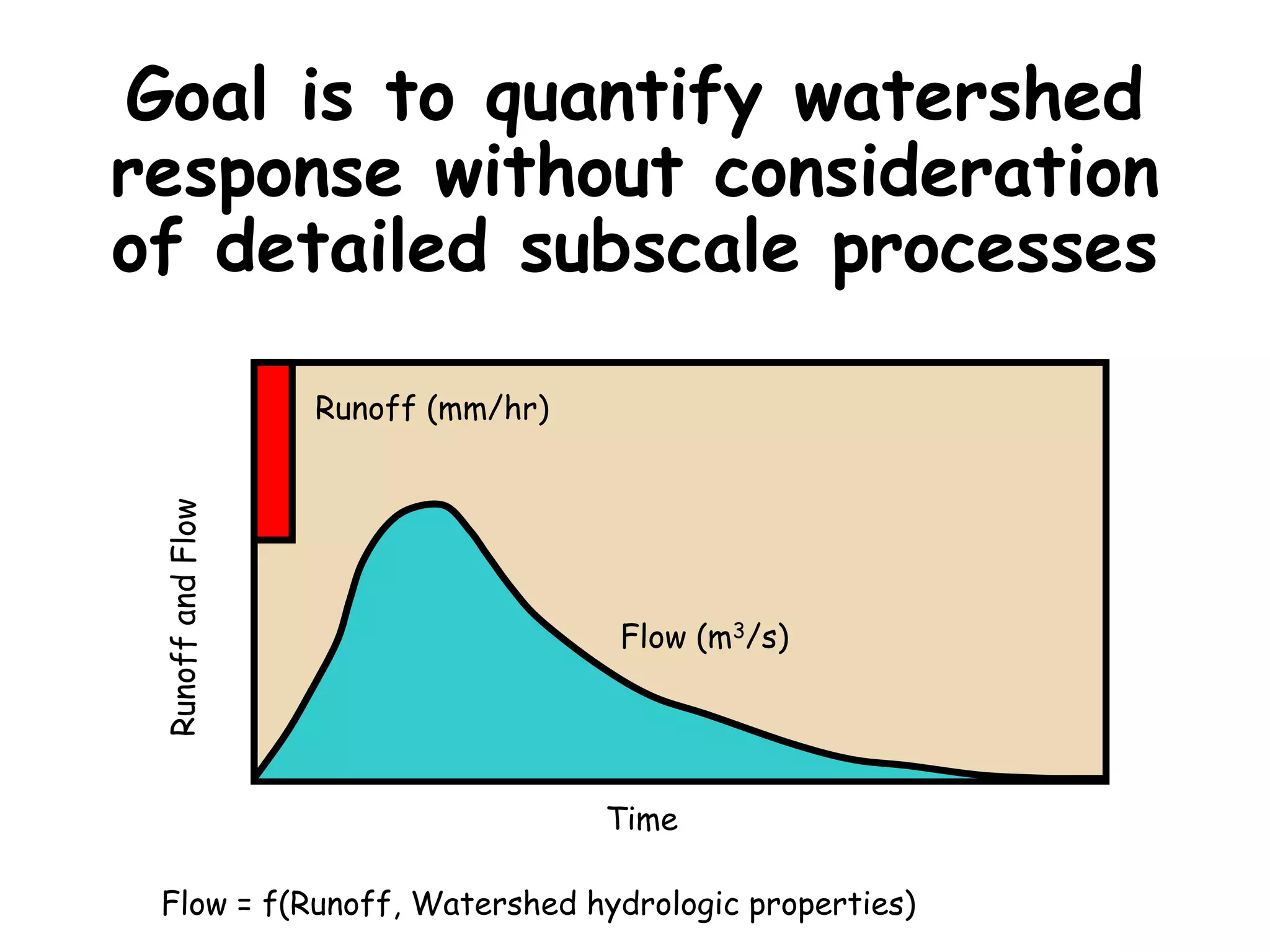
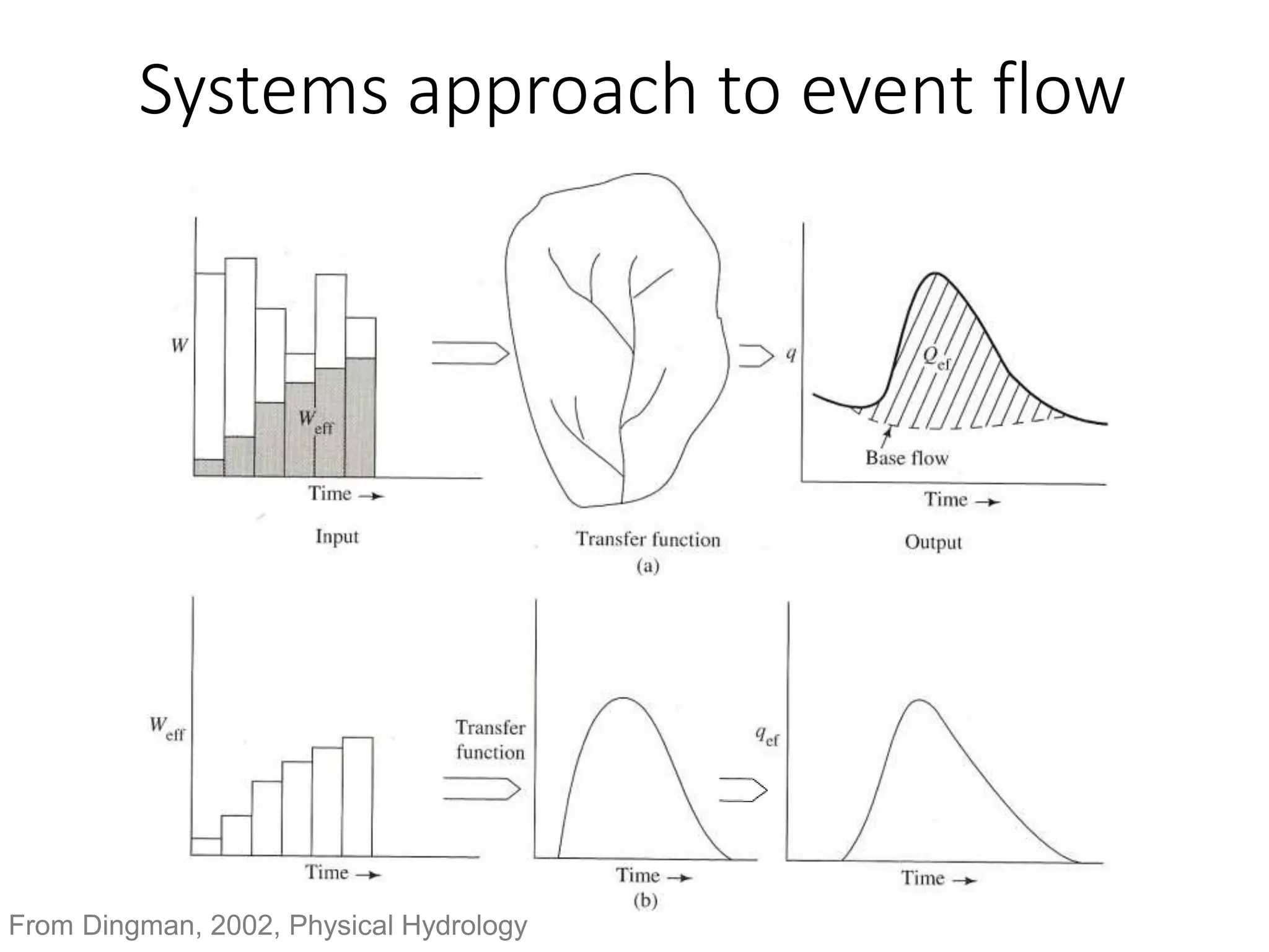
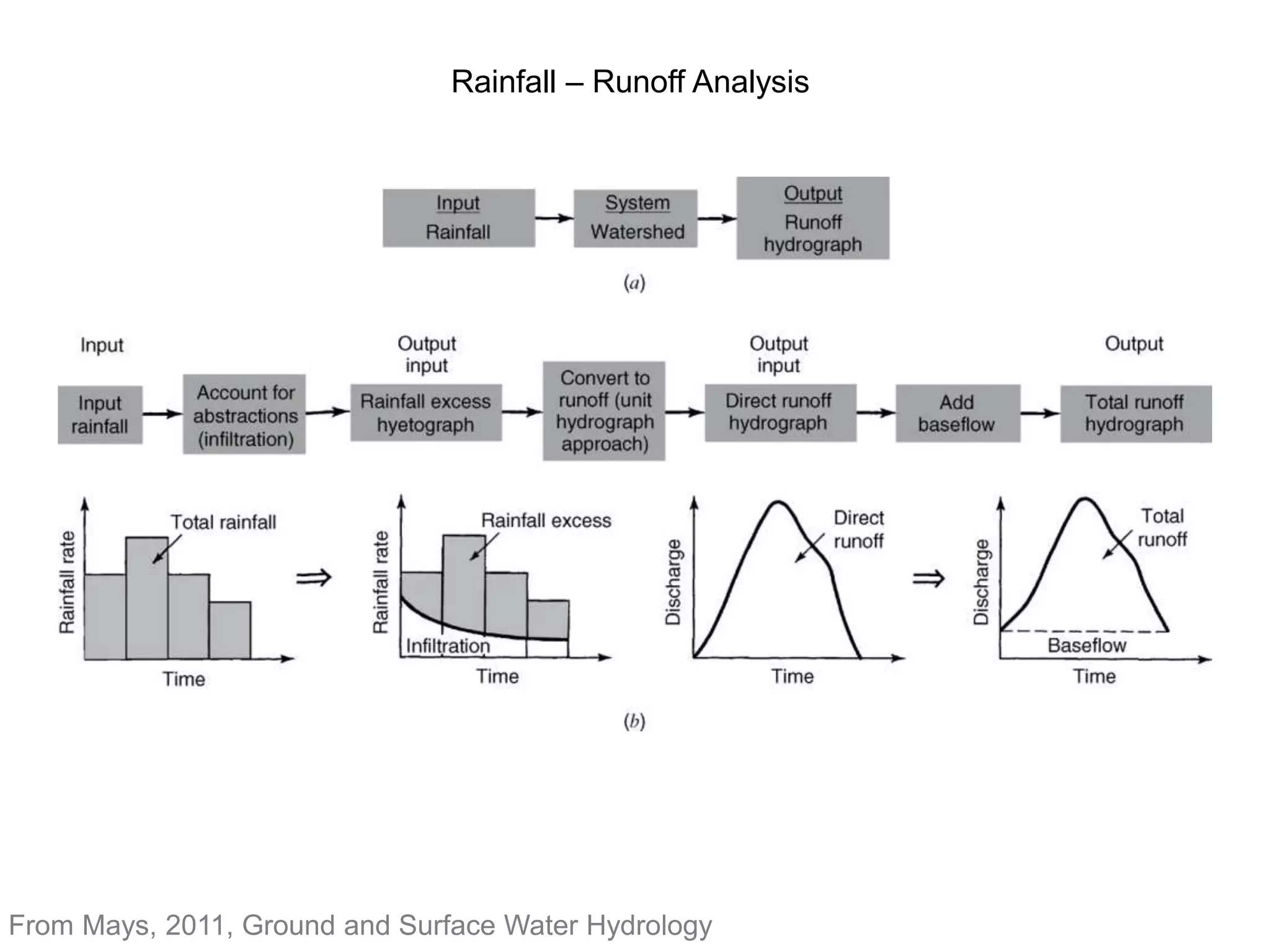
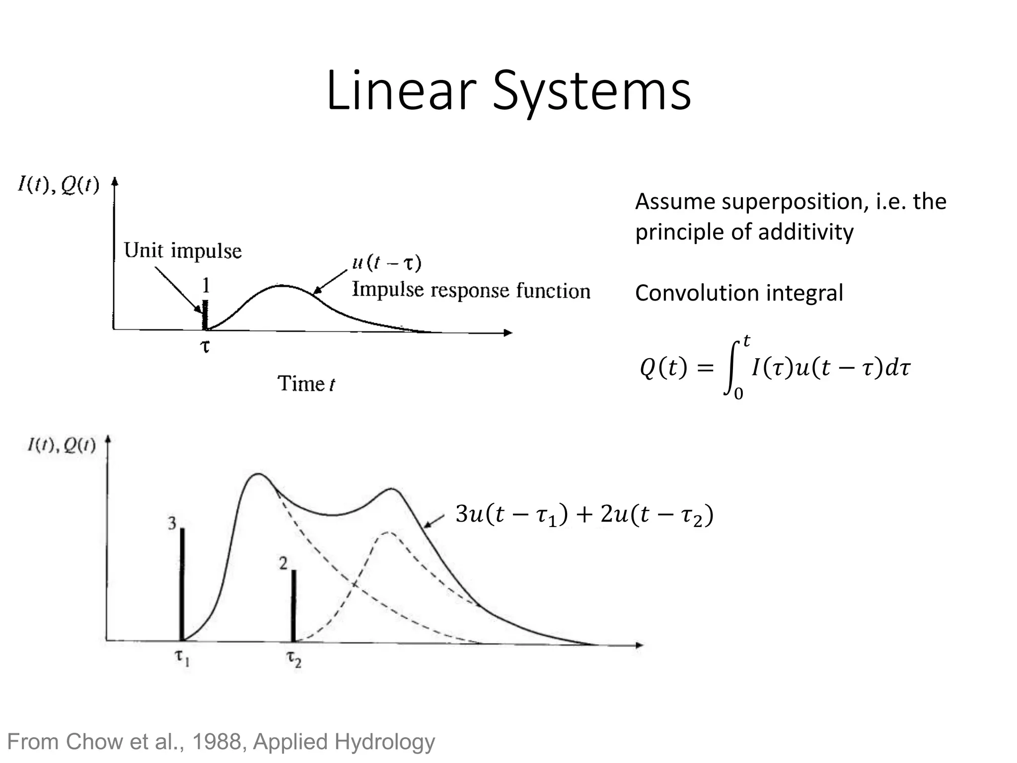
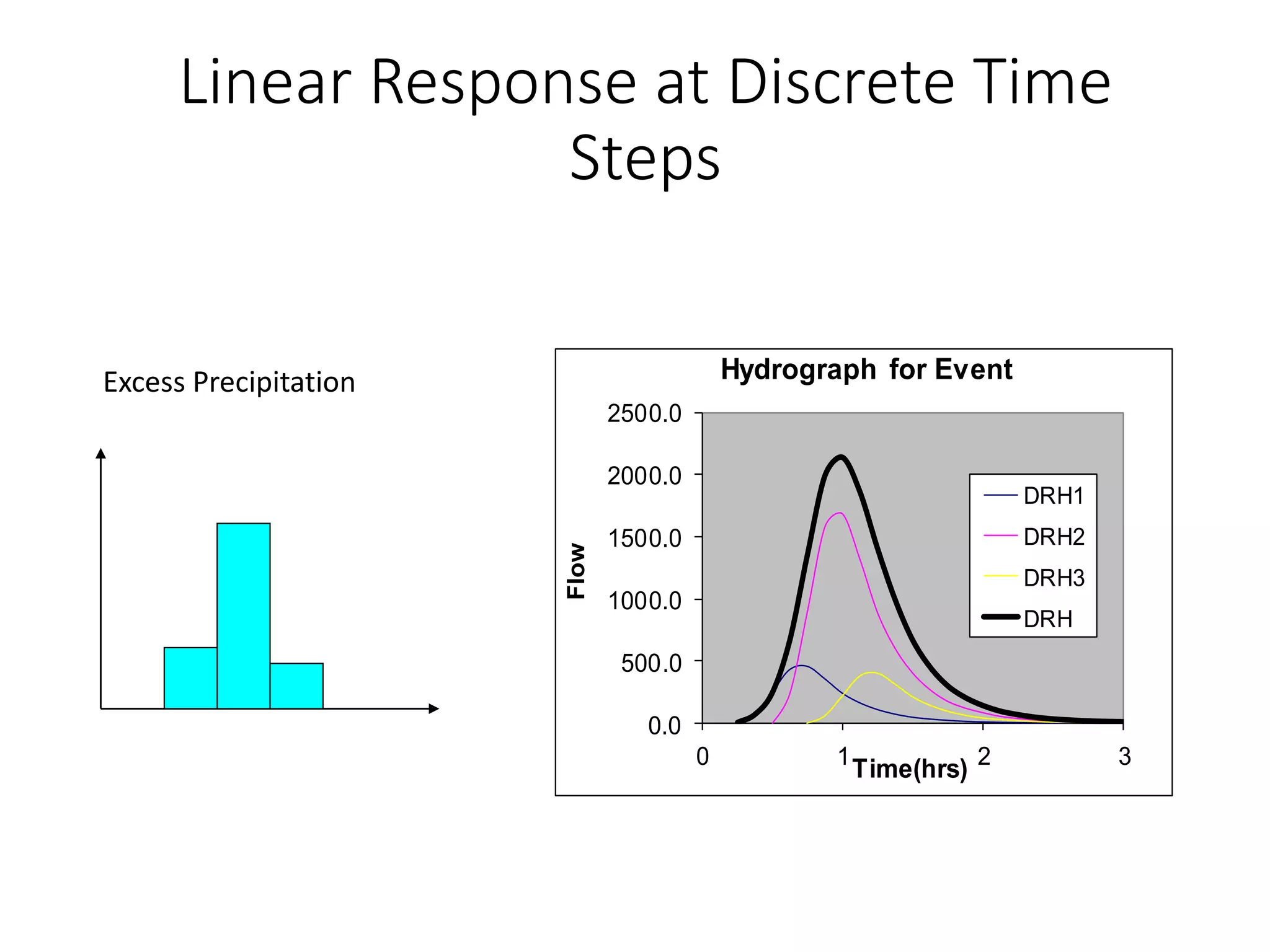
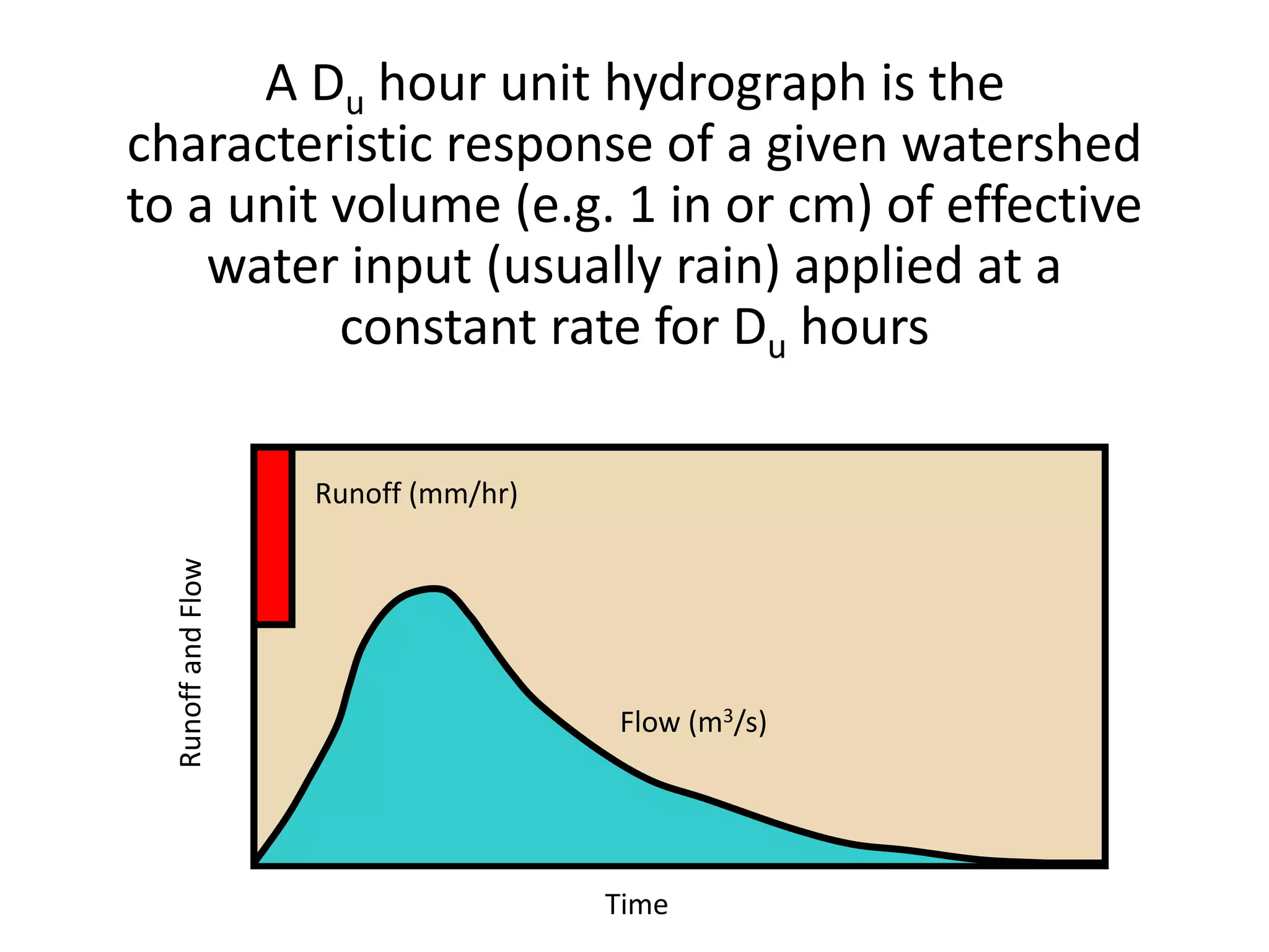
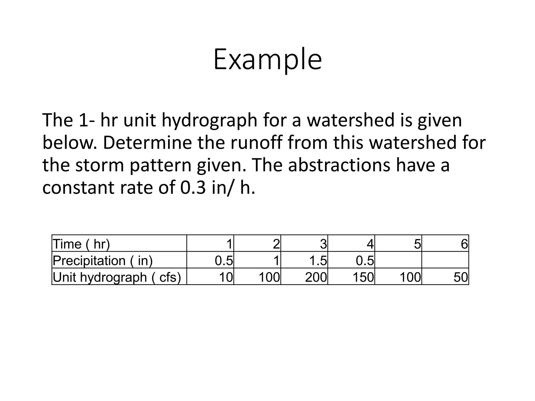
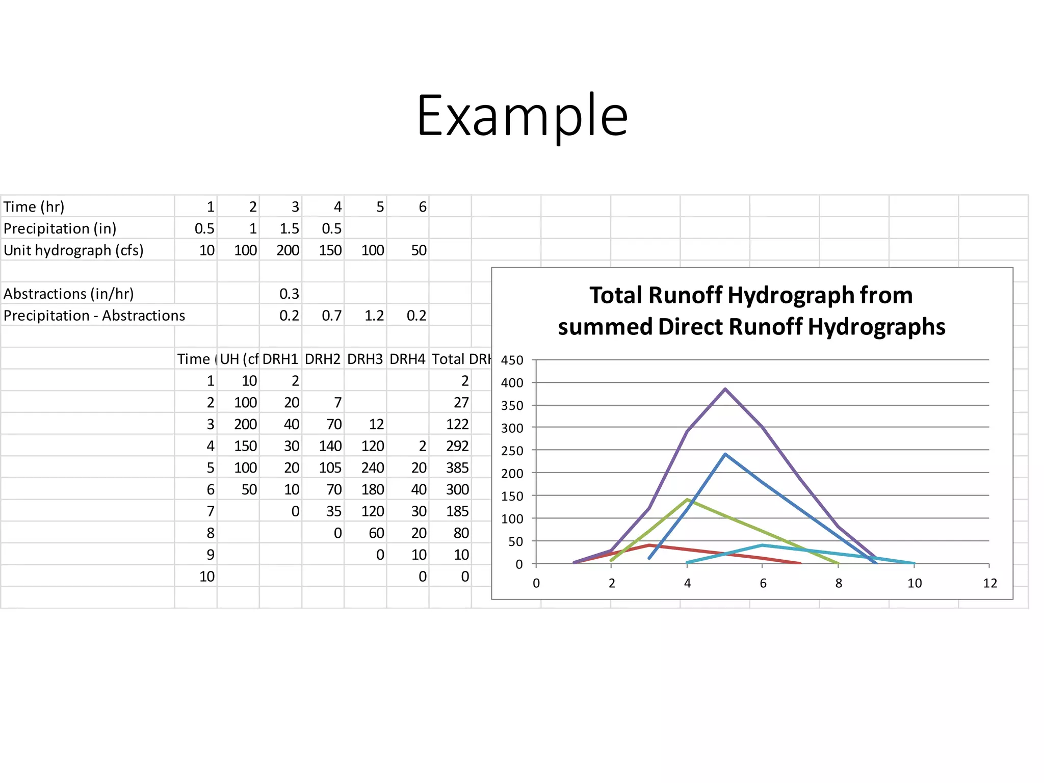
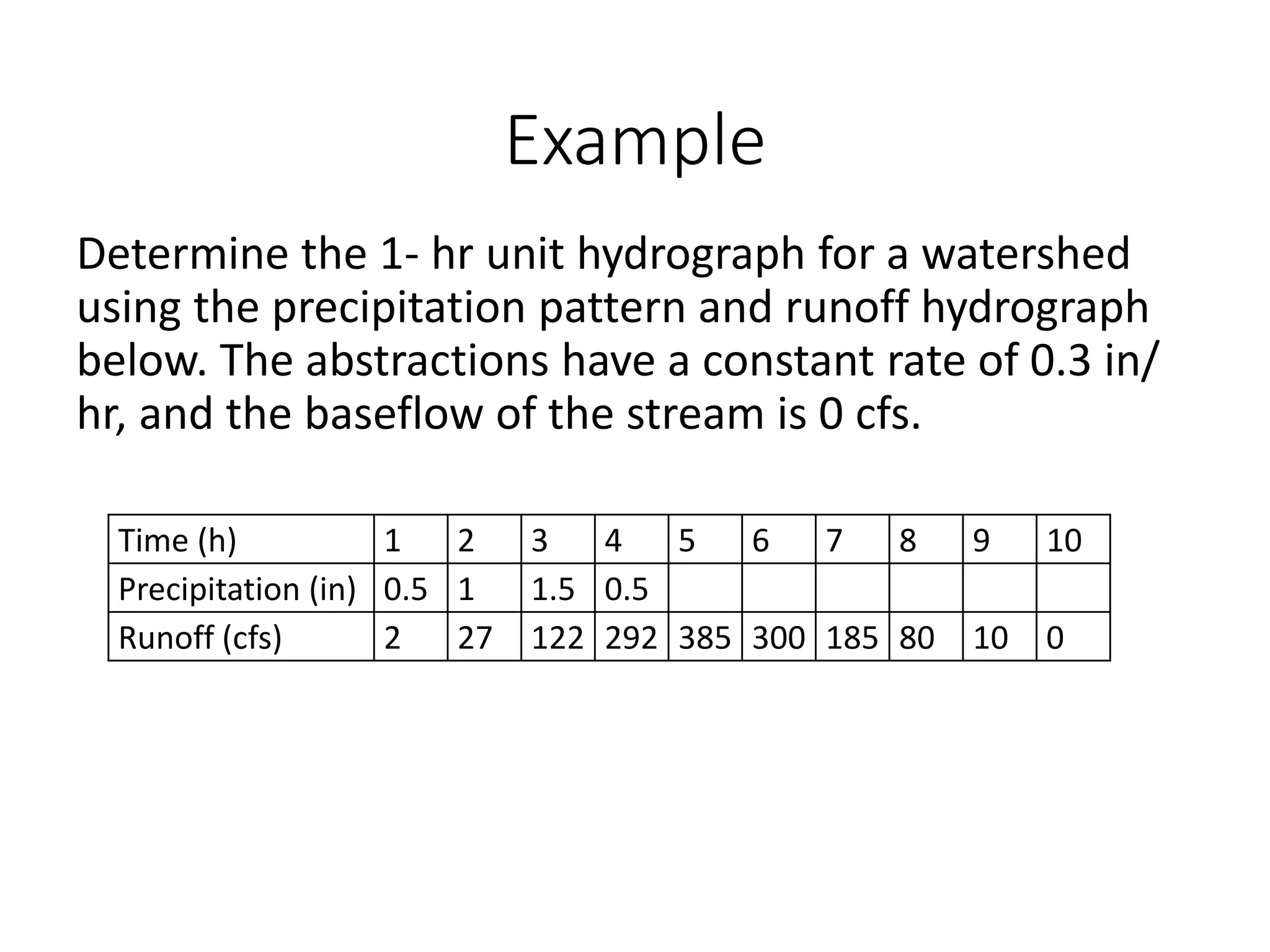
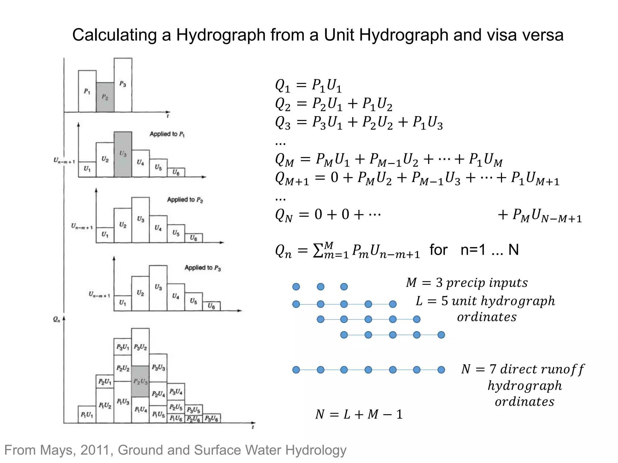
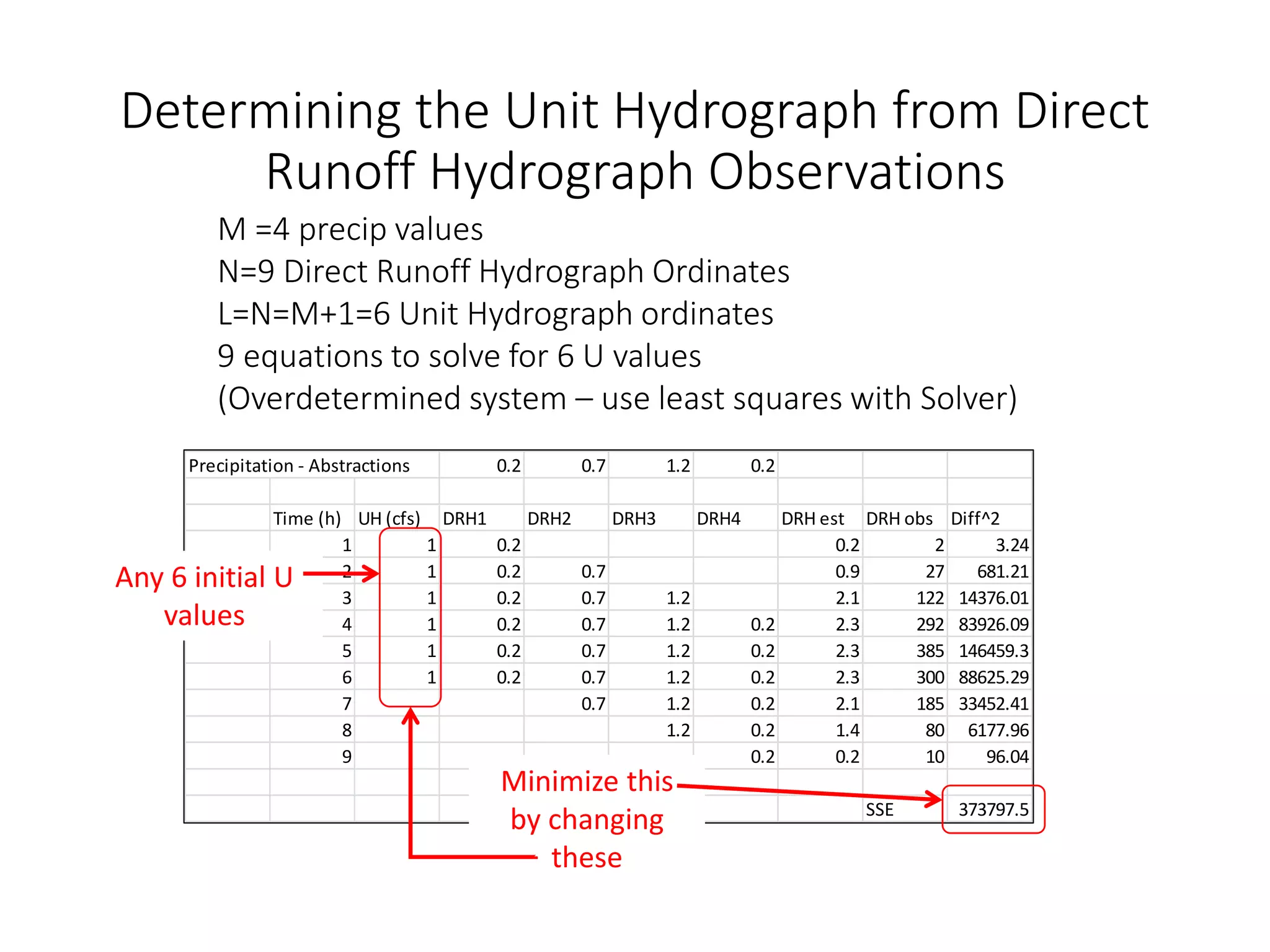
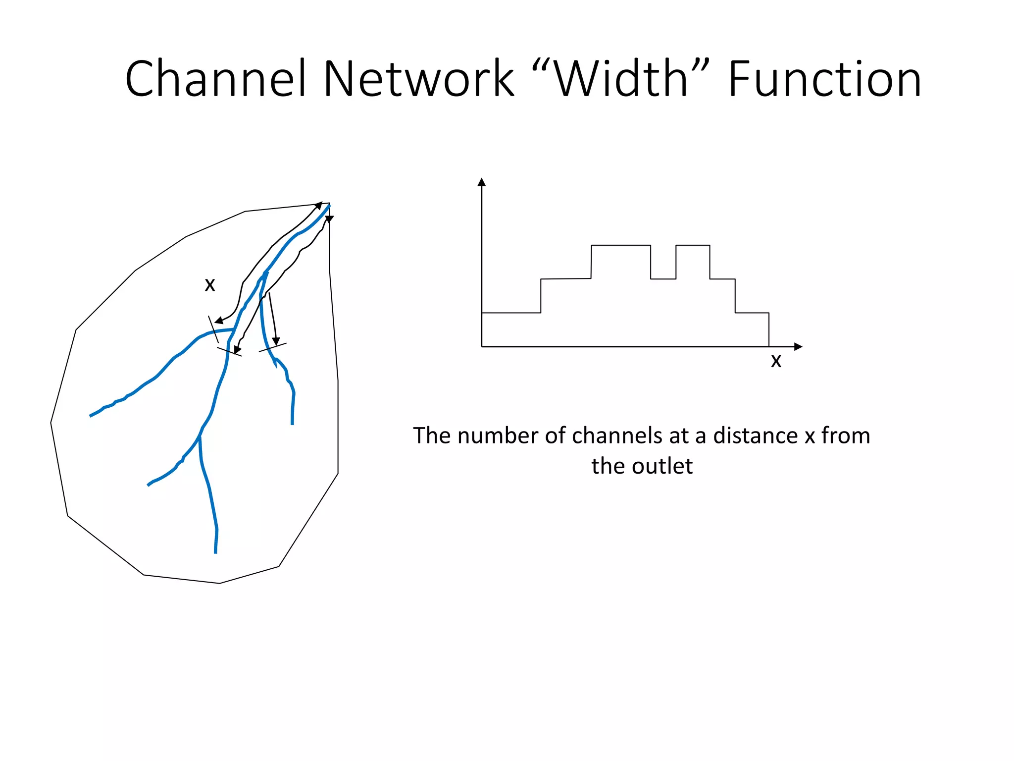
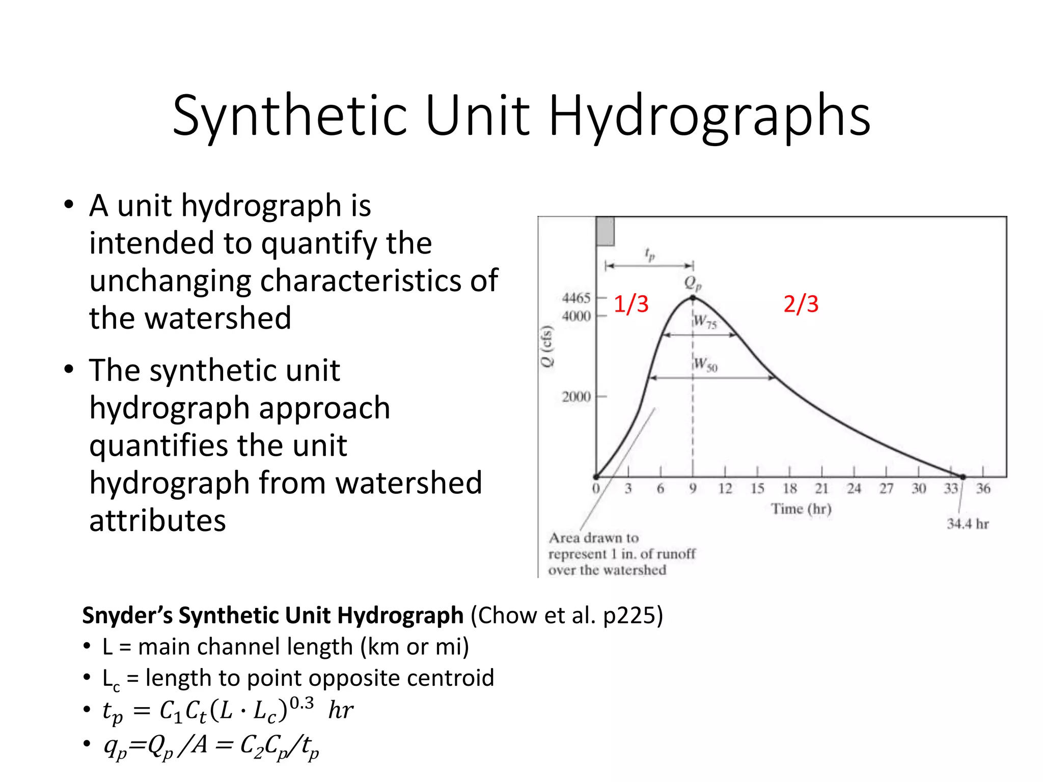
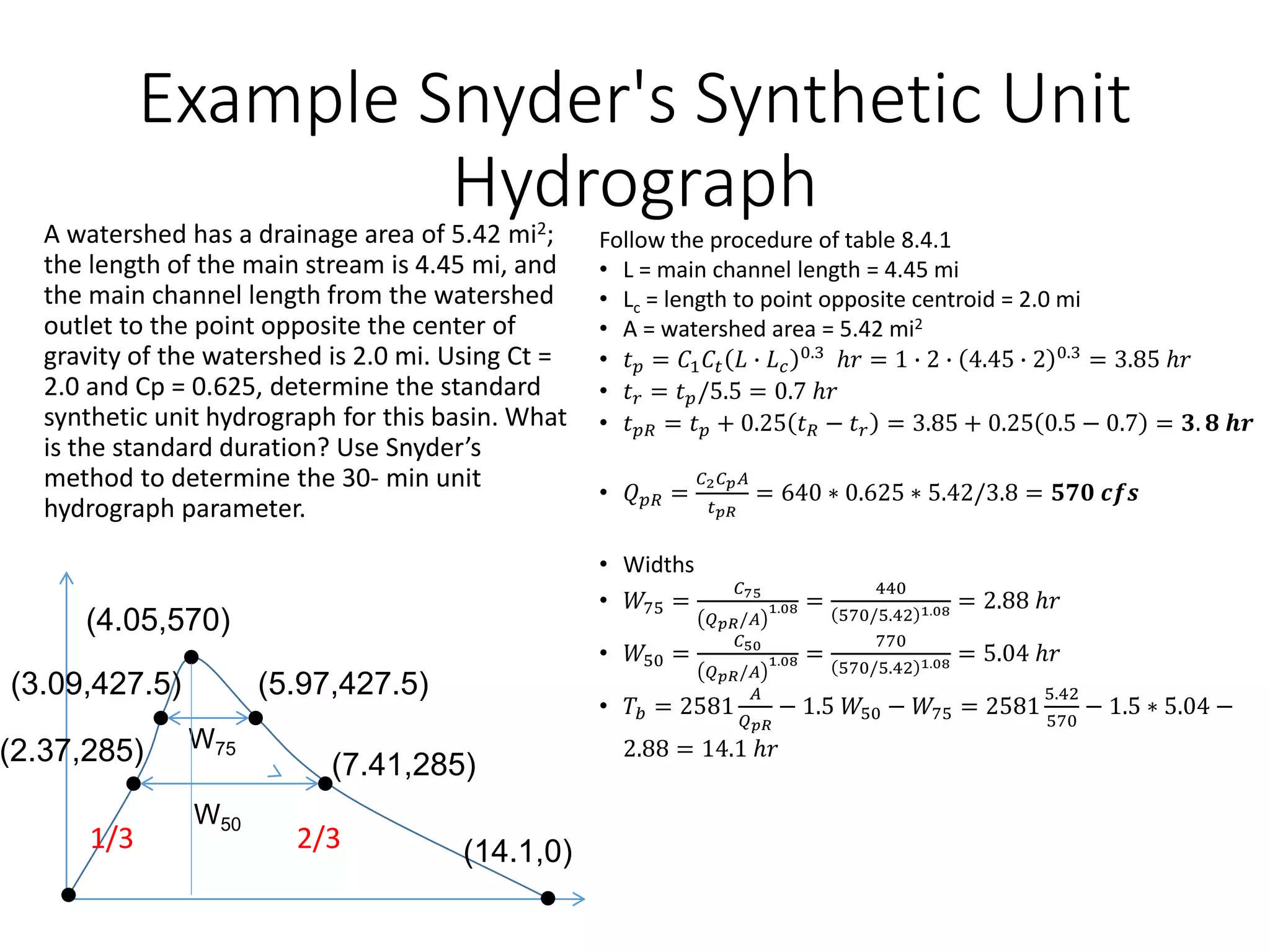
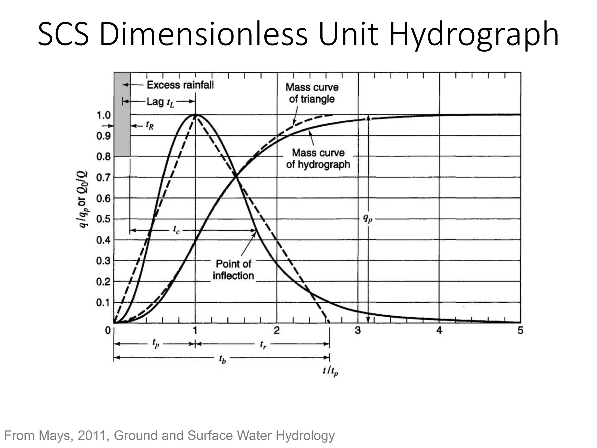
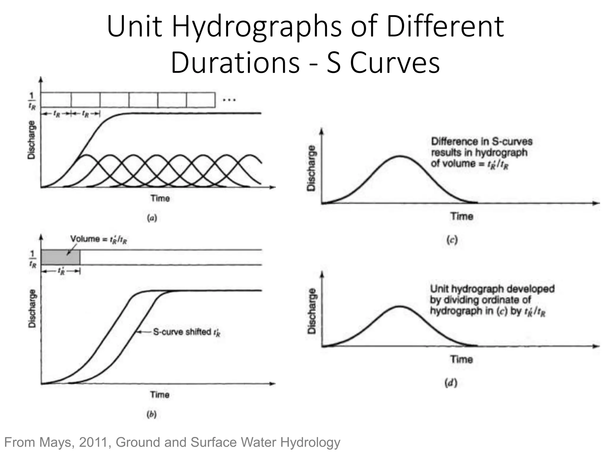
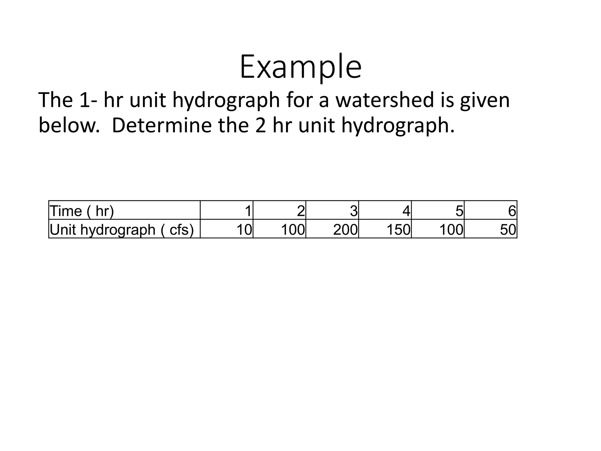
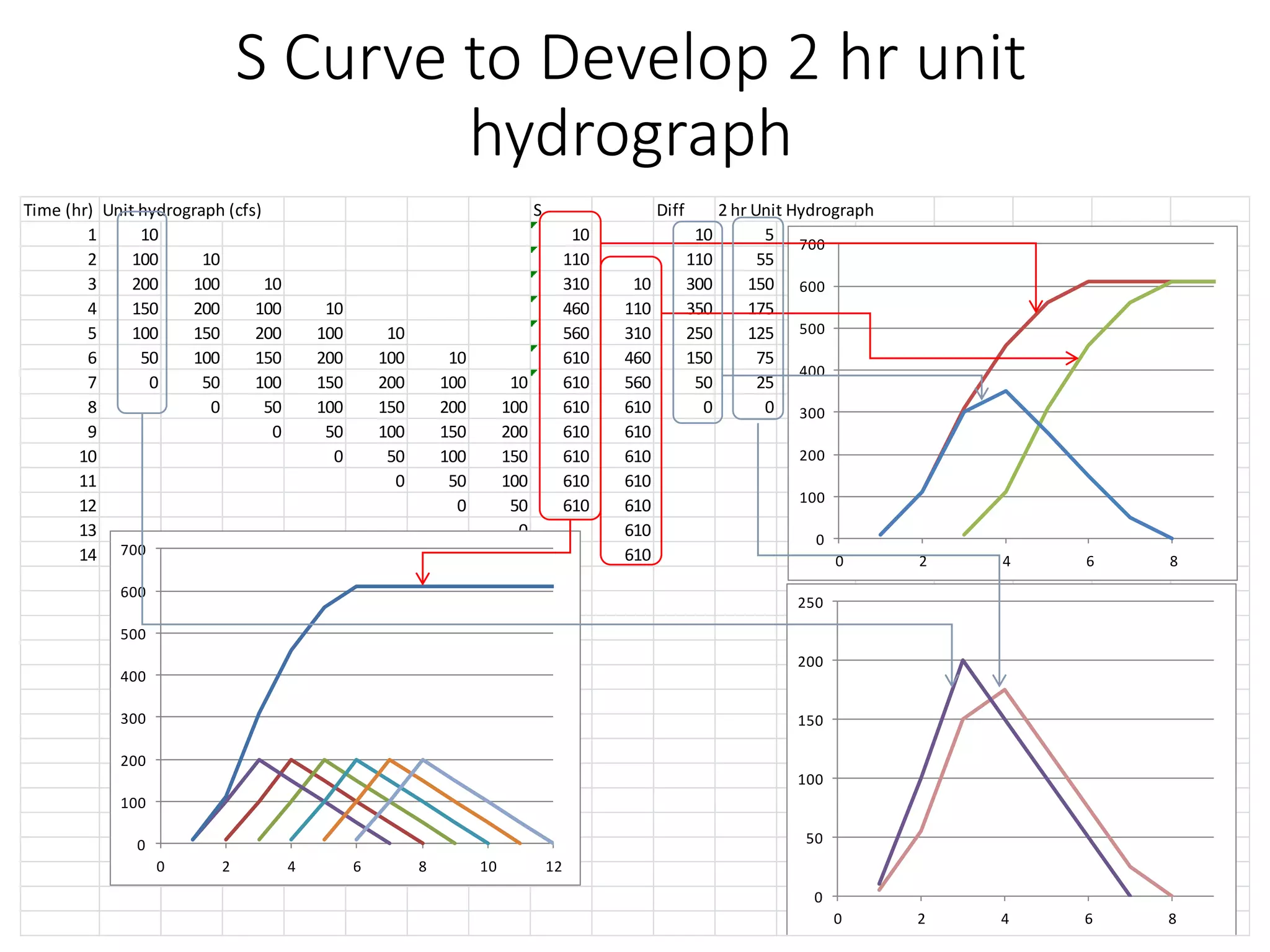
Routing surface runoff to a basin
outlet
Learning objectives
• Be able to use stationary linear response methods
(unit hydrograph) to calculate catchment response
• Be able to estimate the unit hydrograph from data
• Be able to describe the assumptions, limitations and
uses of linear response methods
Chow, V. T., D. R. Maidment and L. W. Mays, (1988), Applied
Hydrology, McGraw Hill, 572 p. Chapter 7
Goal is to quantify watershed
response without consideration
of detailed subscale processes
Runoff (mm/hr)
Flow (m3/s)
Time
Flow = f(Runoff, Watershed hydrologic properties)
Systems approach to event flow
From Dingman, 2002, Physical Hydrology
Rainfall – Runoff Analysis
From Mays, 2011, Ground and Surface Water Hydrology
Linear Systems
3𝑢 𝑡 − 𝜏1 + 2𝑢(𝑡 − 𝜏2)
𝑄 𝑡 =
0
𝑡
𝐼 𝜏 𝑢 𝑡 − 𝜏 𝑑𝜏
From Chow et al., 1988, Applied Hydrology
Assume superposition, i.e. the
principle of additivity
Convolution integral
Linear Response at Discrete Time
Steps
Excess Precipitation
0.0
500.0
1000.0
1500.0
2000.0
2500.0
0 1 2 3
Flow
Time(hrs)
Hydrograph for Event
DRH1
DRH2
DRH3
DRH
A Du hour unit hydrograph is the
characteristic response of a given watershed
to a unit volume (e.g. 1 in or cm) of effective
water input (usually rain) applied at a
constant rate for Du hours
Runoff (mm/hr)
Flow (m3/s)
Time
Assumptions (Chow P 214)
• Excess rainfall has constant intensity within effective
duration
• Excess rainfall is uniformly distributed over watershed
• The base time of the direct runoff hydrograph from
an increment of excess rainfall is constant
• The ordinates of all direct runoff hydrographs are
proportional to the amount of direct runoff
• For a given watershed the hydrograph resulting from
a given excess rainfall reflects the unchanging
characteristics of the watershed
Calculating a Hydrograph from a Unit Hydrograph
𝑄1 = 𝑃1𝑈1
𝑄2 = 𝑃2𝑈1 + 𝑃1𝑈2
𝑄3 = 𝑃3𝑈1 + 𝑃2𝑈2 + 𝑃1𝑈3
...
𝑄𝑀 = 𝑃𝑀𝑈1 + 𝑃𝑀−1𝑈2 + ⋯ + 𝑃1𝑈𝑀
𝑄𝑀+1 = 0 + 𝑃𝑀𝑈2 + 𝑃𝑀−1𝑈3 + ⋯ + 𝑃1𝑈𝑀+1
...
𝑄𝑁 = 0 + 0 + ⋯ + 𝑃𝑀𝑈𝑁−𝑀+1
𝑄𝑛 = 𝑚=1
𝑀
𝑃𝑚𝑈𝑛−𝑚+1 for n=1 ... N
From Mays, 2011, Ground and Surface Water Hydrology
Chow page 217
Example
The 1- hr unit hydrograph for a watershed is given
below. Determine the runoff from this watershed for
the storm pattern given. The abstractions have a
constant rate of 0.3 in/ h.
Time ( hr) 1 2 3 4 5 6
Precipitation ( in) 0.5 1 1.5 0.5
Unit hydrograph ( cfs) 10 100 200 150 100 50
Example
Time (hr) 1 2 3 4 5 6
Precipitation (in) 0.5 1 1.5 0.5
Unit hydrograph (cfs) 10 100 200 150 100 50
Abstractions (in/hr) 0.3
Precipitation - Abstractions 0.2 0.7 1.2 0.2
Time (h)
UH (cfs)
DRH1 DRH2 DRH3 DRH4 Total DRH
1 10 2 2
2 100 20 7 27
3 200 40 70 12 122
4 150 30 140 120 2 292
5 100 20 105 240 20 385
6 50 10 70 180 40 300
7 0 35 120 30 185
8 0 60 20 80
9 0 10 10
10 0 0
0
50
100
150
200
250
300
350
400
450
0 2 4 6 8 10 12
Total Runoff Hydrograph from
summed Direct Runoff Hydrographs
Limitations
• Linearity is violated when deeper water flows
faster.
• Rainfall is seldom uniform in space
• Effective input is very uncertain and depends on
antecedent conditions
Example
Determine the 1- hr unit hydrograph for a watershed
using the precipitation pattern and runoff hydrograph
below. The abstractions have a constant rate of 0.3 in/
hr, and the baseflow of the stream is 0 cfs.
Time (h) 1 2 3 4 5 6 7 8 9 10
Precipitation (in) 0.5 1 1.5 0.5
Runoff (cfs) 2 27 122 292 385 300 185 80 10 0
Calculating a Hydrograph from a Unit Hydrograph and visa versa
𝑄1 = 𝑃1𝑈1
𝑄2 = 𝑃2𝑈1 + 𝑃1𝑈2
𝑄3 = 𝑃3𝑈1 + 𝑃2𝑈2 + 𝑃1𝑈3
...
𝑄𝑀 = 𝑃𝑀𝑈1 + 𝑃𝑀−1𝑈2 + ⋯ + 𝑃1𝑈𝑀
𝑄𝑀+1 = 0 + 𝑃𝑀𝑈2 + 𝑃𝑀−1𝑈3 + ⋯ + 𝑃1𝑈𝑀+1
...
𝑄𝑁 = 0 + 0 + ⋯ + 𝑃𝑀𝑈𝑁−𝑀+1
𝑄𝑛 = 𝑚=1
𝑀
𝑃𝑚𝑈𝑛−𝑚+1 for n=1 ... N
From Mays, 2011, Ground and Surface Water Hydrology
𝑀 = 3 𝑝𝑟𝑒𝑐𝑖𝑝 𝑖𝑛𝑝𝑢𝑡𝑠
𝐿 = 5 𝑢𝑛𝑖𝑡 ℎ𝑦𝑑𝑟𝑜𝑔𝑟𝑎𝑝ℎ
𝑜𝑟𝑑𝑖𝑛𝑎𝑡𝑒𝑠
𝑁 = 7 𝑑𝑖𝑟𝑒𝑐𝑡 𝑟𝑢𝑛𝑜𝑓𝑓
ℎ𝑦𝑑𝑟𝑜𝑔𝑟𝑎𝑝ℎ
𝑜𝑟𝑑𝑖𝑛𝑎𝑡𝑒𝑠
𝑁 = 𝐿 + 𝑀 − 1
Determining the Unit Hydrograph from Direct
Runoff Hydrograph Observations
Precipitation - Abstractions 0.2 0.7 1.2 0.2
Time (h) UH (cfs) DRH1 DRH2 DRH3 DRH4 DRH est DRH obs Diff^2
1 1 0.2 0.2 2 3.24
2 1 0.2 0.7 0.9 27 681.21
3 1 0.2 0.7 1.2 2.1 122 14376.01
4 1 0.2 0.7 1.2 0.2 2.3 292 83926.09
5 1 0.2 0.7 1.2 0.2 2.3 385 146459.3
6 1 0.2 0.7 1.2 0.2 2.3 300 88625.29
7 0.7 1.2 0.2 2.1 185 33452.41
8 1.2 0.2 1.4 80 6177.96
9 0.2 0.2 10 96.04
SSE 373797.5
M =4 precip values
N=9 Direct Runoff Hydrograph Ordinates
L=N=M+1=6 Unit Hydrograph ordinates
9 equations to solve for 6 U values
(Overdetermined system – use least squares with Solver)
Any 6 initial U
values
Minimize this
by changing
these
Which hydrograph is associated
with each watershed
1
2
3
A
B
C
Time Area Diagram
Distribution function of area by travel time to
outlet
Under assumptions of constant velocity
t = d/v
This provides a geomorphological basis for defining
the unit response function.
Channel Network “Width” Function
The number of channels at a distance x from
the outlet
x
x
Synthetic Unit Hydrographs
• A unit hydrograph is
intended to quantify the
unchanging characteristics of
the watershed
• The synthetic unit
hydrograph approach
quantifies the unit
hydrograph from watershed
attributes
1/3 2/3
Snyder’s Synthetic Unit Hydrograph (Chow et al. p225)
• L = main channel length (km or mi)
• Lc = length to point opposite centroid
• 𝑡𝑝 = 𝐶1𝐶𝑡 𝐿 ∙ 𝐿𝑐
0.3 ℎ𝑟
• qp=Qp /A = C2Cp/tp
Example Snyder's Synthetic Unit
Hydrograph
A watershed has a drainage area of 5.42 mi2;
the length of the main stream is 4.45 mi, and
the main channel length from the watershed
outlet to the point opposite the center of
gravity of the watershed is 2.0 mi. Using Ct =
2.0 and Cp = 0.625, determine the standard
synthetic unit hydrograph for this basin. What
is the standard duration? Use Snyder’s
method to determine the 30- min unit
hydrograph parameter.
Follow the procedure of table 8.4.1
• L = main channel length = 4.45 mi
• Lc = length to point opposite centroid = 2.0 mi
• A = watershed area = 5.42 mi2
• 𝑡𝑝 = 𝐶1𝐶𝑡 𝐿 ∙ 𝐿𝑐
0.3
ℎ𝑟 = 1 ∙ 2 ∙ 4.45 ∙ 2 0.3
= 3.85 ℎ𝑟
• 𝑡𝑟 = 𝑡𝑝/5.5 = 0.7 ℎ𝑟
• 𝑡𝑝𝑅 = 𝑡𝑝 + 0.25 𝑡𝑅 − 𝑡𝑟 = 3.85 + 0.25 0.5 − 0.7 = 𝟑. 𝟖 𝒉𝒓
• 𝑄𝑝𝑅 =
𝐶2𝐶𝑝𝐴
𝑡𝑝𝑅
= 640 ∗ 0.625 ∗ 5.42/3.8 = 𝟓𝟕𝟎 𝒄𝒇𝒔
• Widths
• 𝑊75 =
𝐶75
𝑄𝑝𝑅/𝐴
1.08 =
440
570/5.42 1.08 = 2.88 ℎ𝑟
• 𝑊50 =
𝐶50
𝑄𝑝𝑅/𝐴
1.08 =
770
570/5.42 1.08 = 5.04 ℎ𝑟
• 𝑇𝑏 = 2581
𝐴
𝑄𝑝𝑅
− 1.5 𝑊50 − 𝑊75 = 2581
5.42
570
− 1.5 ∗ 5.04 −
2.88 = 14.1 ℎ𝑟
(2.37,285)
(3.09,427.5)
(4.05,570)
(5.97,427.5)
(7.41,285)
(14.1,0)
W50
W75
1/3 2/3
SCS Dimensionless Unit Hydrograph
From Mays, 2011, Ground and Surface Water Hydrology
Unit Hydrographs of Different
Durations - S Curves
From Mays, 2011, Ground and Surface Water Hydrology
Example
The 1- hr unit hydrograph for a watershed is given
below. Determine the 2 hr unit hydrograph.
Time ( hr) 1 2 3 4 5 6
Unit hydrograph ( cfs) 10 100 200 150 100 50
S Curve to Develop 2 hr unit
hydrograph
Time (hr) Unit hydrograph (cfs) S Diff 2 hr Unit Hydrograph
1 10 10 10 5
2 100 10 110 110 55
3 200 100 10 310 10 300 150
4 150 200 100 10 460 110 350 175
5 100 150 200 100 10 560 310 250 125
6 50 100 150 200 100 10 610 460 150 75
7 0 50 100 150 200 100 10 610 560 50 25
8 0 50 100 150 200 100 610 610 0 0
9 0 50 100 150 200 610 610
10 0 50 100 150 610 610
11 0 50 100 610 610
12 0 50 610 610
13 0 610
14 610
0
100
200
300
400
500
600
700
0 2 4 6 8
0
100
200
300
400
500
600
700
0 2 4 6 8 10 12
0
50
100
150
200
250
0 2 4 6 8

UnitHydrograph.pptx

  • 1.
    Routing surface runoffto a basin outlet Learning objectives • Be able to use stationary linear response methods (unit hydrograph) to calculate catchment response • Be able to estimate the unit hydrograph from data • Be able to describe the assumptions, limitations and uses of linear response methods Chow, V. T., D. R. Maidment and L. W. Mays, (1988), Applied Hydrology, McGraw Hill, 572 p. Chapter 7
  • 2.
    Goal is toquantify watershed response without consideration of detailed subscale processes Runoff (mm/hr) Flow (m3/s) Time Flow = f(Runoff, Watershed hydrologic properties)
  • 3.
    Systems approach toevent flow From Dingman, 2002, Physical Hydrology
  • 4.
    Rainfall – RunoffAnalysis From Mays, 2011, Ground and Surface Water Hydrology
  • 5.
    Linear Systems 3𝑢 𝑡− 𝜏1 + 2𝑢(𝑡 − 𝜏2) 𝑄 𝑡 = 0 𝑡 𝐼 𝜏 𝑢 𝑡 − 𝜏 𝑑𝜏 From Chow et al., 1988, Applied Hydrology Assume superposition, i.e. the principle of additivity Convolution integral
  • 6.
    Linear Response atDiscrete Time Steps Excess Precipitation 0.0 500.0 1000.0 1500.0 2000.0 2500.0 0 1 2 3 Flow Time(hrs) Hydrograph for Event DRH1 DRH2 DRH3 DRH
  • 7.
    A Du hourunit hydrograph is the characteristic response of a given watershed to a unit volume (e.g. 1 in or cm) of effective water input (usually rain) applied at a constant rate for Du hours Runoff (mm/hr) Flow (m3/s) Time
  • 8.
    Assumptions (Chow P214) • Excess rainfall has constant intensity within effective duration • Excess rainfall is uniformly distributed over watershed • The base time of the direct runoff hydrograph from an increment of excess rainfall is constant • The ordinates of all direct runoff hydrographs are proportional to the amount of direct runoff • For a given watershed the hydrograph resulting from a given excess rainfall reflects the unchanging characteristics of the watershed
  • 9.
    Calculating a Hydrographfrom a Unit Hydrograph 𝑄1 = 𝑃1𝑈1 𝑄2 = 𝑃2𝑈1 + 𝑃1𝑈2 𝑄3 = 𝑃3𝑈1 + 𝑃2𝑈2 + 𝑃1𝑈3 ... 𝑄𝑀 = 𝑃𝑀𝑈1 + 𝑃𝑀−1𝑈2 + ⋯ + 𝑃1𝑈𝑀 𝑄𝑀+1 = 0 + 𝑃𝑀𝑈2 + 𝑃𝑀−1𝑈3 + ⋯ + 𝑃1𝑈𝑀+1 ... 𝑄𝑁 = 0 + 0 + ⋯ + 𝑃𝑀𝑈𝑁−𝑀+1 𝑄𝑛 = 𝑚=1 𝑀 𝑃𝑚𝑈𝑛−𝑚+1 for n=1 ... N From Mays, 2011, Ground and Surface Water Hydrology Chow page 217
  • 10.
    Example The 1- hrunit hydrograph for a watershed is given below. Determine the runoff from this watershed for the storm pattern given. The abstractions have a constant rate of 0.3 in/ h. Time ( hr) 1 2 3 4 5 6 Precipitation ( in) 0.5 1 1.5 0.5 Unit hydrograph ( cfs) 10 100 200 150 100 50
  • 11.
    Example Time (hr) 12 3 4 5 6 Precipitation (in) 0.5 1 1.5 0.5 Unit hydrograph (cfs) 10 100 200 150 100 50 Abstractions (in/hr) 0.3 Precipitation - Abstractions 0.2 0.7 1.2 0.2 Time (h) UH (cfs) DRH1 DRH2 DRH3 DRH4 Total DRH 1 10 2 2 2 100 20 7 27 3 200 40 70 12 122 4 150 30 140 120 2 292 5 100 20 105 240 20 385 6 50 10 70 180 40 300 7 0 35 120 30 185 8 0 60 20 80 9 0 10 10 10 0 0 0 50 100 150 200 250 300 350 400 450 0 2 4 6 8 10 12 Total Runoff Hydrograph from summed Direct Runoff Hydrographs
  • 12.
    Limitations • Linearity isviolated when deeper water flows faster. • Rainfall is seldom uniform in space • Effective input is very uncertain and depends on antecedent conditions
  • 13.
    Example Determine the 1-hr unit hydrograph for a watershed using the precipitation pattern and runoff hydrograph below. The abstractions have a constant rate of 0.3 in/ hr, and the baseflow of the stream is 0 cfs. Time (h) 1 2 3 4 5 6 7 8 9 10 Precipitation (in) 0.5 1 1.5 0.5 Runoff (cfs) 2 27 122 292 385 300 185 80 10 0
  • 14.
    Calculating a Hydrographfrom a Unit Hydrograph and visa versa 𝑄1 = 𝑃1𝑈1 𝑄2 = 𝑃2𝑈1 + 𝑃1𝑈2 𝑄3 = 𝑃3𝑈1 + 𝑃2𝑈2 + 𝑃1𝑈3 ... 𝑄𝑀 = 𝑃𝑀𝑈1 + 𝑃𝑀−1𝑈2 + ⋯ + 𝑃1𝑈𝑀 𝑄𝑀+1 = 0 + 𝑃𝑀𝑈2 + 𝑃𝑀−1𝑈3 + ⋯ + 𝑃1𝑈𝑀+1 ... 𝑄𝑁 = 0 + 0 + ⋯ + 𝑃𝑀𝑈𝑁−𝑀+1 𝑄𝑛 = 𝑚=1 𝑀 𝑃𝑚𝑈𝑛−𝑚+1 for n=1 ... N From Mays, 2011, Ground and Surface Water Hydrology 𝑀 = 3 𝑝𝑟𝑒𝑐𝑖𝑝 𝑖𝑛𝑝𝑢𝑡𝑠 𝐿 = 5 𝑢𝑛𝑖𝑡 ℎ𝑦𝑑𝑟𝑜𝑔𝑟𝑎𝑝ℎ 𝑜𝑟𝑑𝑖𝑛𝑎𝑡𝑒𝑠 𝑁 = 7 𝑑𝑖𝑟𝑒𝑐𝑡 𝑟𝑢𝑛𝑜𝑓𝑓 ℎ𝑦𝑑𝑟𝑜𝑔𝑟𝑎𝑝ℎ 𝑜𝑟𝑑𝑖𝑛𝑎𝑡𝑒𝑠 𝑁 = 𝐿 + 𝑀 − 1
  • 15.
    Determining the UnitHydrograph from Direct Runoff Hydrograph Observations Precipitation - Abstractions 0.2 0.7 1.2 0.2 Time (h) UH (cfs) DRH1 DRH2 DRH3 DRH4 DRH est DRH obs Diff^2 1 1 0.2 0.2 2 3.24 2 1 0.2 0.7 0.9 27 681.21 3 1 0.2 0.7 1.2 2.1 122 14376.01 4 1 0.2 0.7 1.2 0.2 2.3 292 83926.09 5 1 0.2 0.7 1.2 0.2 2.3 385 146459.3 6 1 0.2 0.7 1.2 0.2 2.3 300 88625.29 7 0.7 1.2 0.2 2.1 185 33452.41 8 1.2 0.2 1.4 80 6177.96 9 0.2 0.2 10 96.04 SSE 373797.5 M =4 precip values N=9 Direct Runoff Hydrograph Ordinates L=N=M+1=6 Unit Hydrograph ordinates 9 equations to solve for 6 U values (Overdetermined system – use least squares with Solver) Any 6 initial U values Minimize this by changing these
  • 16.
    Which hydrograph isassociated with each watershed 1 2 3 A B C
  • 17.
    Time Area Diagram Distributionfunction of area by travel time to outlet Under assumptions of constant velocity t = d/v This provides a geomorphological basis for defining the unit response function.
  • 18.
    Channel Network “Width”Function The number of channels at a distance x from the outlet x x
  • 19.
    Synthetic Unit Hydrographs •A unit hydrograph is intended to quantify the unchanging characteristics of the watershed • The synthetic unit hydrograph approach quantifies the unit hydrograph from watershed attributes 1/3 2/3 Snyder’s Synthetic Unit Hydrograph (Chow et al. p225) • L = main channel length (km or mi) • Lc = length to point opposite centroid • 𝑡𝑝 = 𝐶1𝐶𝑡 𝐿 ∙ 𝐿𝑐 0.3 ℎ𝑟 • qp=Qp /A = C2Cp/tp
  • 20.
    Example Snyder's SyntheticUnit Hydrograph A watershed has a drainage area of 5.42 mi2; the length of the main stream is 4.45 mi, and the main channel length from the watershed outlet to the point opposite the center of gravity of the watershed is 2.0 mi. Using Ct = 2.0 and Cp = 0.625, determine the standard synthetic unit hydrograph for this basin. What is the standard duration? Use Snyder’s method to determine the 30- min unit hydrograph parameter. Follow the procedure of table 8.4.1 • L = main channel length = 4.45 mi • Lc = length to point opposite centroid = 2.0 mi • A = watershed area = 5.42 mi2 • 𝑡𝑝 = 𝐶1𝐶𝑡 𝐿 ∙ 𝐿𝑐 0.3 ℎ𝑟 = 1 ∙ 2 ∙ 4.45 ∙ 2 0.3 = 3.85 ℎ𝑟 • 𝑡𝑟 = 𝑡𝑝/5.5 = 0.7 ℎ𝑟 • 𝑡𝑝𝑅 = 𝑡𝑝 + 0.25 𝑡𝑅 − 𝑡𝑟 = 3.85 + 0.25 0.5 − 0.7 = 𝟑. 𝟖 𝒉𝒓 • 𝑄𝑝𝑅 = 𝐶2𝐶𝑝𝐴 𝑡𝑝𝑅 = 640 ∗ 0.625 ∗ 5.42/3.8 = 𝟓𝟕𝟎 𝒄𝒇𝒔 • Widths • 𝑊75 = 𝐶75 𝑄𝑝𝑅/𝐴 1.08 = 440 570/5.42 1.08 = 2.88 ℎ𝑟 • 𝑊50 = 𝐶50 𝑄𝑝𝑅/𝐴 1.08 = 770 570/5.42 1.08 = 5.04 ℎ𝑟 • 𝑇𝑏 = 2581 𝐴 𝑄𝑝𝑅 − 1.5 𝑊50 − 𝑊75 = 2581 5.42 570 − 1.5 ∗ 5.04 − 2.88 = 14.1 ℎ𝑟 (2.37,285) (3.09,427.5) (4.05,570) (5.97,427.5) (7.41,285) (14.1,0) W50 W75 1/3 2/3
  • 21.
    SCS Dimensionless UnitHydrograph From Mays, 2011, Ground and Surface Water Hydrology
  • 22.
    Unit Hydrographs ofDifferent Durations - S Curves From Mays, 2011, Ground and Surface Water Hydrology
  • 23.
    Example The 1- hrunit hydrograph for a watershed is given below. Determine the 2 hr unit hydrograph. Time ( hr) 1 2 3 4 5 6 Unit hydrograph ( cfs) 10 100 200 150 100 50
  • 24.
    S Curve toDevelop 2 hr unit hydrograph Time (hr) Unit hydrograph (cfs) S Diff 2 hr Unit Hydrograph 1 10 10 10 5 2 100 10 110 110 55 3 200 100 10 310 10 300 150 4 150 200 100 10 460 110 350 175 5 100 150 200 100 10 560 310 250 125 6 50 100 150 200 100 10 610 460 150 75 7 0 50 100 150 200 100 10 610 560 50 25 8 0 50 100 150 200 100 610 610 0 0 9 0 50 100 150 200 610 610 10 0 50 100 150 610 610 11 0 50 100 610 610 12 0 50 610 610 13 0 610 14 610 0 100 200 300 400 500 600 700 0 2 4 6 8 0 100 200 300 400 500 600 700 0 2 4 6 8 10 12 0 50 100 150 200 250 0 2 4 6 8