PREDICTION OF THE FLOW REGIME IN THE
ABSENCE OF THE DISCHARGE DATA
ACKNOWLEDGEMENT
 I would like to express my deep sense of gratitude,
indebtedness and sincere thanks to my guide professor
Dr. Basudev biswal , assistant professor civil
engineering at IIT Hyderabad for his invaluable
guidance, support and encouragement during the
course of my work. I would also like to take this
opportunity to put on record my respect to Anita nag
{research scholar, IIT Hyderabad}for providing me
moral support during the completion of my work.
ABSTRACT
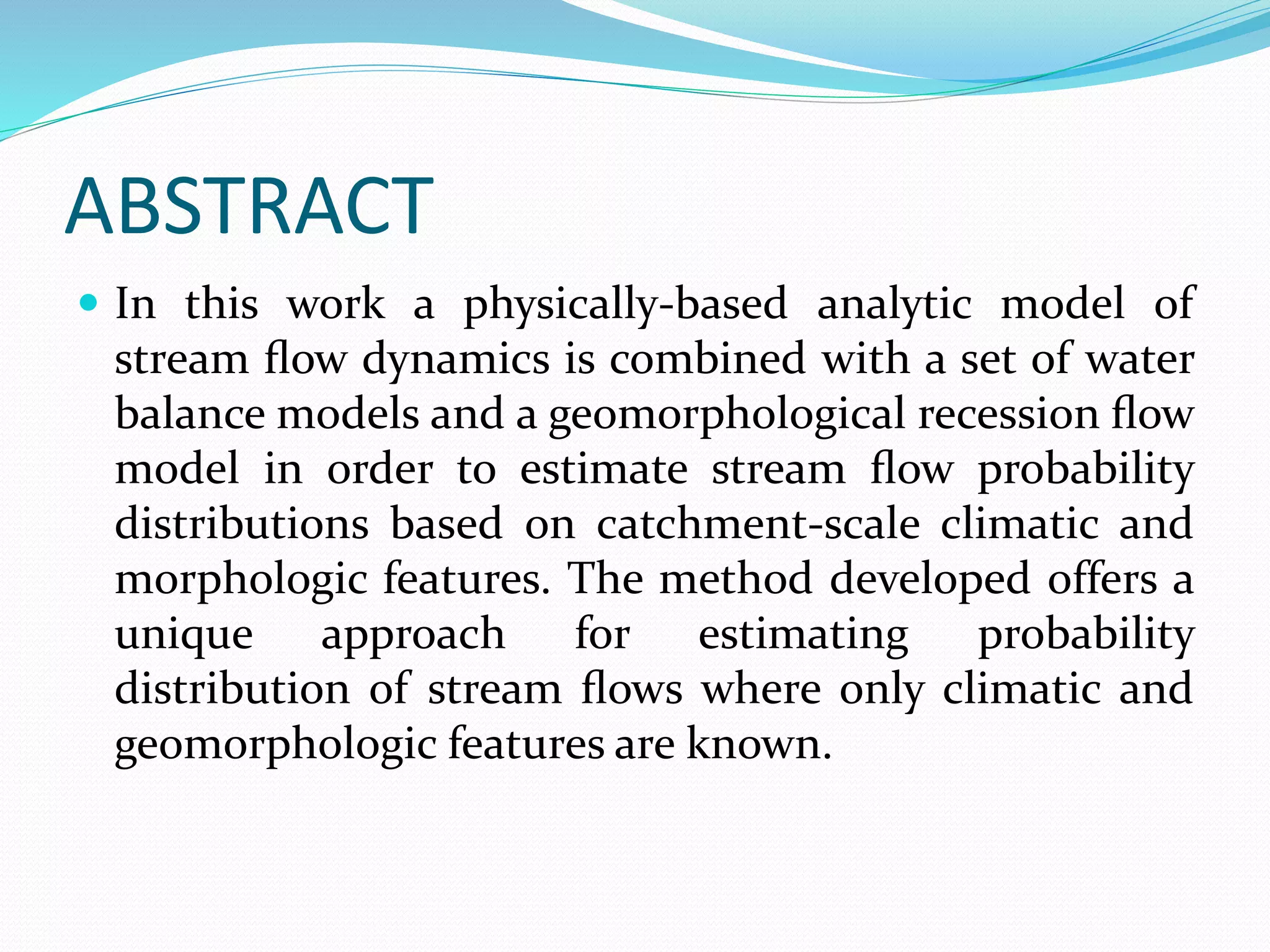
 In this work a physically-based analytic model of
stream flow dynamics is combined with a set of water
balance models and a geomorphological recession flow
model in order to estimate stream flow probability
distributions based on catchment-scale climatic and
morphologic features. The method developed offers a
unique approach for estimating probability
distribution of stream flows where only climatic and
geomorphologic features are known.
 This method was developed by Botter . This is a
mechanistic approach where the dynamics of daily
stream flow are linked to a spatially integrated soil
water balance forced by intermittent rainfall.
 It adopts the version of the model in which the
hydrologic response of the catchment is assumed to be
non linear.
 The four physically based parameters that define the
flow duration curve are estimated based on climatic
data {rainfall, potential evapotranspiration} and
geomorphological data{DEMs} which integrates into
established water balance models and geomorphic
recession flow models{GRFM}
 WATER BALANCE MODEL
 Regarding this model , a number of catchments are
selected which are divided into two sets:-
1. Calibration catchment
2. Test catchment
 Calibration catchments are basically used for the
calibration of the water balance models.
 Test catchments are the catchments where stream flow
distribution were predicted using climatic and
morphological data.
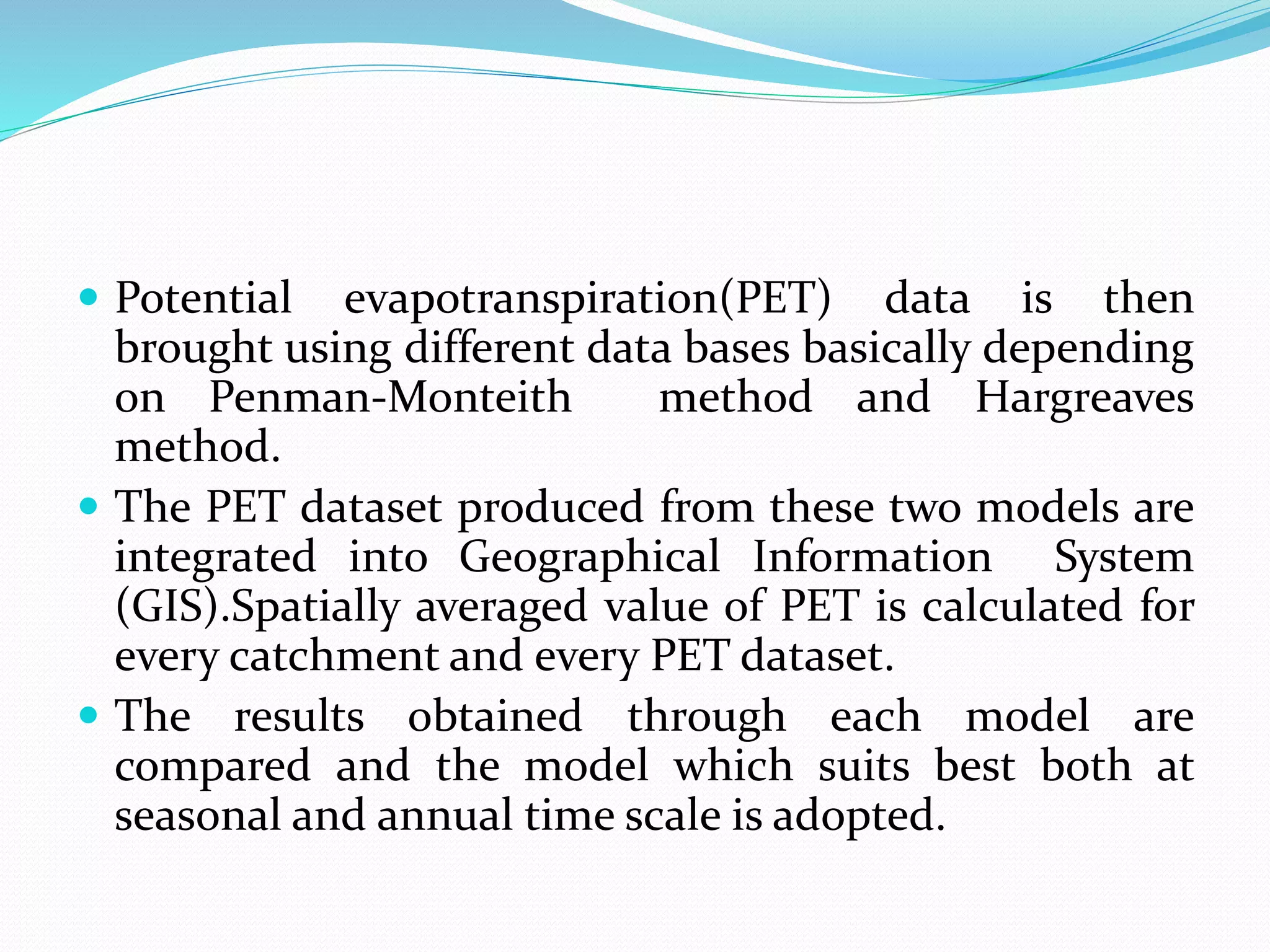
 Potential evapotranspiration(PET) data is then
brought using different data bases basically depending
on Penman-Monteith method and Hargreaves
method.
 The PET dataset produced from these two models are
integrated into Geographical Information System
(GIS).Spatially averaged value of PET is calculated for
every catchment and every PET dataset.
 The results obtained through each model are
compared and the model which suits best both at
seasonal and annual time scale is adopted.
 The contributing catchments and drainage network
upstream of discharge gauging station are then
estimated.
 The river flow regime can be characterized by the
seasonal Probability Density Function (PDF) of daily
stream flows which is described through the analytical
mechanistic model developed by Botter et al.
 This mechanistic model is based on catchment scale
soil water balance forced by stochastic rainfall which is
modeled as marked Poisson process with frequency λ P
and exponentially distributed depth with average α .
 In this method the dynamics of the specific stream
flow Q (per unit catchment area) is made up of two
components:-
(a)Instantaneous jump(effective rainfall) corresponding
to rainfall events filling the soil water deficit in the root
zone . Effective rainfall takes place with frequency λ <
λp and are also represented by Marked Poisson process.
(b) Power laws which decays in between events as
implied by non- linear catchment scale storage
discharge relationship . So temporal dynamics of Q
during a given season is described by the following
relation:-
dQ(t)/dt ={-kQ(t)a}+ξQ(t)
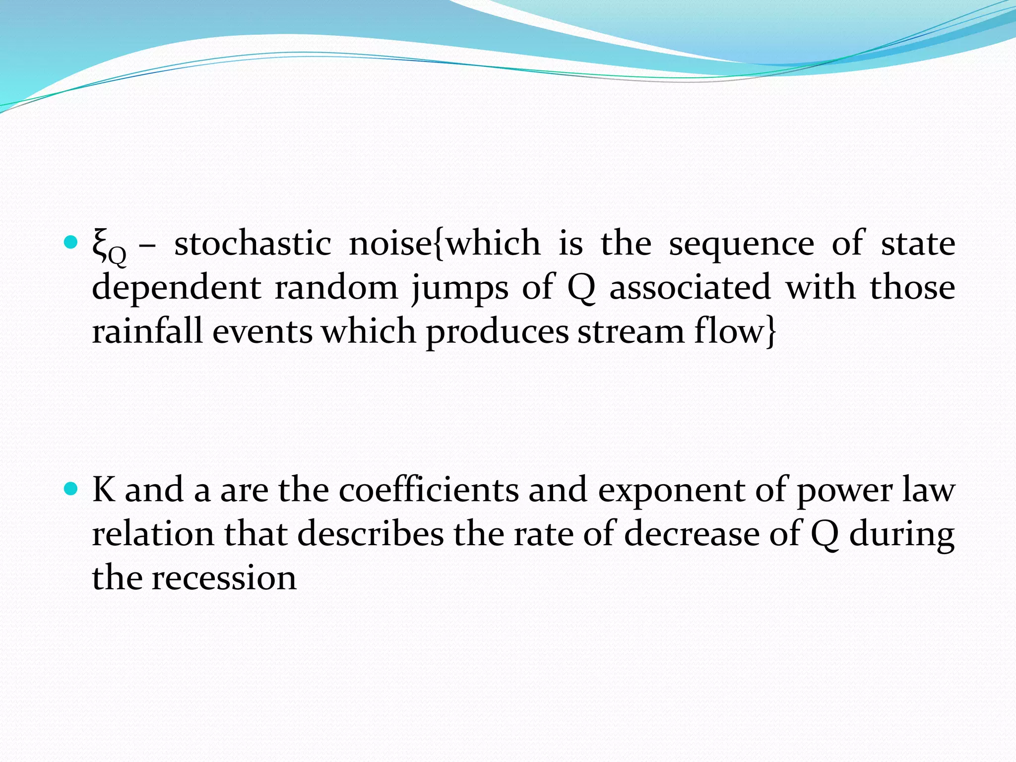
 ξQ – stochastic noise{which is the sequence of state
dependent random jumps of Q associated with those
rainfall events which produces stream flow}
 K and a are the coefficients and exponent of power law
relation that describes the rate of decrease of Q during
the recession
 The steady state PDF (Probability Density Function)
of stream flow can be derived from the solution of the
given equation:-
 P(Q) =CQ-aexp[{Q2-a/αk(2-a)}+{λq1-a/k(1-a)}]
C= suitable normalizing constant
 This master equation expresses the seasonal flow
regime as a function of four physically based
parameters that embed the geomorphic and climatic
feature of contributing catchment.
 FDC is expressed by the cumulative distribution
fraction (CDF) of Q and thus can be calculated as:-
D(Q) = ∫p(x)dx
 Assumptions while carrying out this equation:-
(a) the Poisson distribution of flow producing events.
(b)The exponential distribution of the daily rainfall
and depth
(c)The spatial homogeneity of climate and landscape
properties at the catchment scale.
ESTIMATION OF PARAMETERS
COMPUTATION OF α
 Mean rainfall depth(α) is estimated by means of daily
rainfall data recorded at climatic station within the
boundaries of each catchment . In particular , α is
calculated during wet days when the depth is above
zero.
COMPUTATION OF λ
 λ= Φλp
 Φ=(Q/P)
 Where Φ represents seasonal runoff coefficients
P=αλp
Q=α λ
Φ can be estimated by means of calibrated water
balance models using precipitation and PET data.
COMPUTATION OF a AND k
 These are recession properties that are strongly related
to morphology of the stream network.
 Both the stream flow and Active Drainage Network
(which is nothing but the fraction of the network that
actually contribute to the flow at outlet.) decrease over
time.
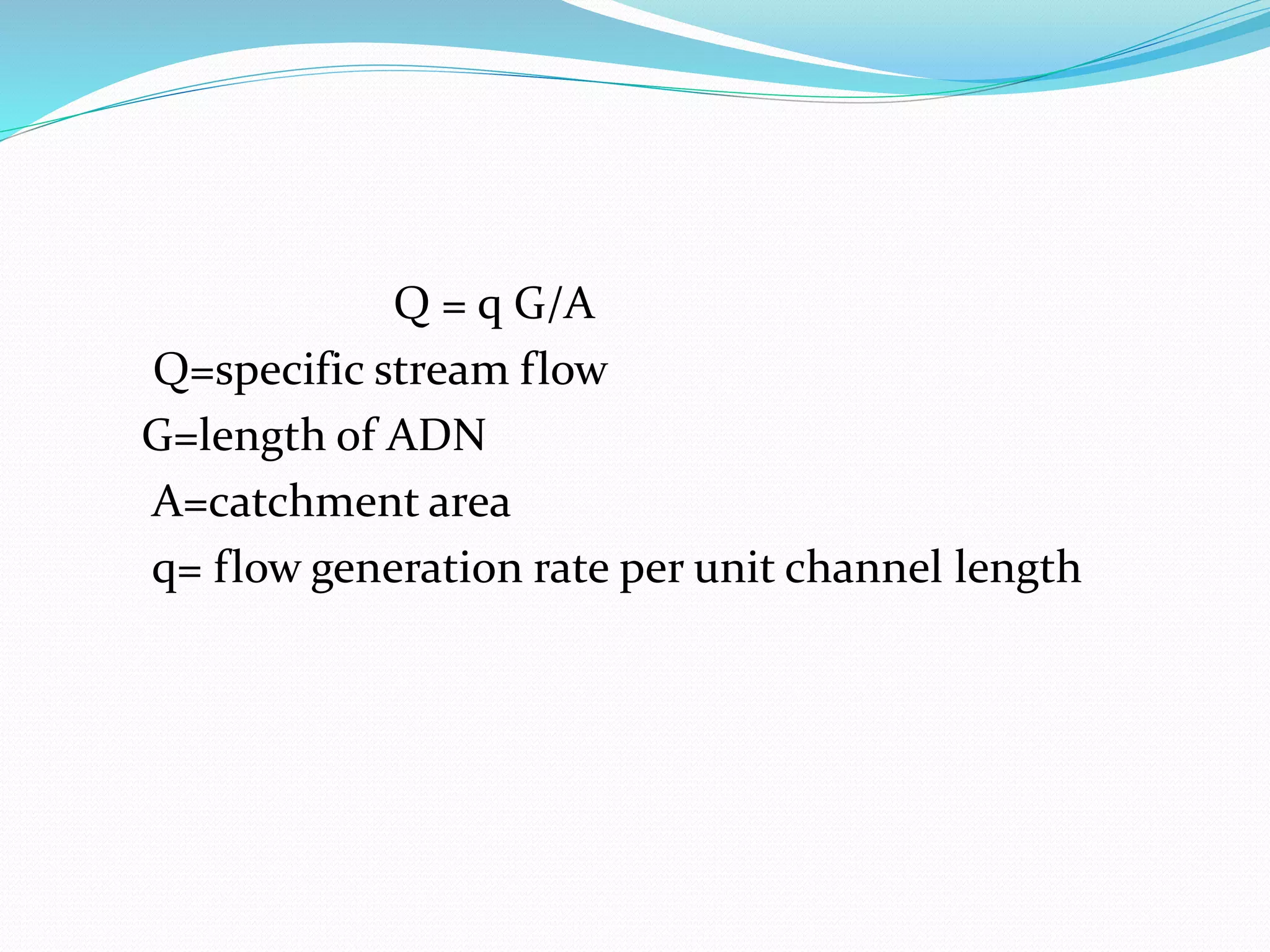
Q = q G/A
Q=specific stream flow
G=length of ADN
A=catchment area
q= flow generation rate per unit channel length
ASSUMPTIONS:-
 Drainage density is assumed spatially uniform
 Both q and speed at which ADN contracts towards the
outlet is constant .
dG/dt=(dG/dl)*(dl/dt)= CdG(l)/dl
The recession equation dQ/dt= kQa can be written as:-
 N(l)/A=ρ’(G(l)/A)a
(1) ρ’=k(q)a-1 /c
 N(l)= dG(l)/dl which represents number
of links in a network at a distance L.
 The equation (1)represents that “a” can be
estimated from the morphology of the basin by
analyzing the scaling exponentof the geomorphic
relationship between N(l) and G(l).This can be
obtained using least square regression .
CALCULATION OF K
 Q= q(G/A) = q Dd
 q= αλ/ Dd
 K=θ (αλ)1-a
OVERVIEW
 The method presented here is structurally able to
provide a reasonable estimation of stream flow
regimes based on limited information about climate
and landscape. This encouraging outcome provides
the opportunity for a number of potential applications
such as evaluation of anthropogenic alteration of flow
regimes or the prediction of hydrologic shifts induced
by climate change.
 The stochastic stream flow model presented here is
best suited to describe flow regimes of pristine
catchments with a contributing area smaller than a few
thousand square kilometers, where stream flow
dynamics result from the interaction between
intermittent precipitation inputs and soil drainage.
 The estimate of the model parameters based on
climate and landscape requires the introduction of
additional assumptions and parameters that may
reduce the accuracy of the flow regime predictions
 The accuracy of the estimate of a (i.e. the degree of
non-linearity of the hydrologic response) based on
catchment morphology may be affected by the
resolution of DEM. Moreover, the estimated value of
‘a’ might depend on the drainage density and its
spatial patterns which can be difficult to assess on
experimental grounds, especially for large catchments.
CONCLUSION
 A method is provided that allows for estimating the
probability distribution of stream flows based on
catchment scale climate and geomorphologic data.
The approach employs a physically-based analytic
model of stream flows with four parameters.
 It was shown that these parameters can be estimated in the
absence of discharge time series, by exploiting climate data
(precipitation, potential evapotranspiration) and
information about the catchment morphology (DEMs).
The estimation procedure required the use of additional
models, which were taken from the literature. A
geomorphologic flow recession model was utilized to
estimate parameters describing the recession behavior of
the hydrograph, based on the topology of the stream
network. A water balance model was used to predict the
frequency of flow producing rainfall events.
THANKS
MOHIT MAYOOR
CUJ/I/2013/IWEM/007
CENTRAL UNIVERSITY OF JHARKHAND

Mechanistic models

  • 1.
    PREDICTION OF THEFLOW REGIME IN THE ABSENCE OF THE DISCHARGE DATA
  • 2.
    ACKNOWLEDGEMENT  I wouldlike to express my deep sense of gratitude, indebtedness and sincere thanks to my guide professor Dr. Basudev biswal , assistant professor civil engineering at IIT Hyderabad for his invaluable guidance, support and encouragement during the course of my work. I would also like to take this opportunity to put on record my respect to Anita nag {research scholar, IIT Hyderabad}for providing me moral support during the completion of my work.
  • 3.
    ABSTRACT  In thiswork a physically-based analytic model of stream flow dynamics is combined with a set of water balance models and a geomorphological recession flow model in order to estimate stream flow probability distributions based on catchment-scale climatic and morphologic features. The method developed offers a unique approach for estimating probability distribution of stream flows where only climatic and geomorphologic features are known.
  • 4.
     This methodwas developed by Botter . This is a mechanistic approach where the dynamics of daily stream flow are linked to a spatially integrated soil water balance forced by intermittent rainfall.  It adopts the version of the model in which the hydrologic response of the catchment is assumed to be non linear.
  • 5.
     The fourphysically based parameters that define the flow duration curve are estimated based on climatic data {rainfall, potential evapotranspiration} and geomorphological data{DEMs} which integrates into established water balance models and geomorphic recession flow models{GRFM}
  • 7.
  • 8.
     Regarding thismodel , a number of catchments are selected which are divided into two sets:- 1. Calibration catchment 2. Test catchment  Calibration catchments are basically used for the calibration of the water balance models.  Test catchments are the catchments where stream flow distribution were predicted using climatic and morphological data.
  • 9.
     Potential evapotranspiration(PET)data is then brought using different data bases basically depending on Penman-Monteith method and Hargreaves method.  The PET dataset produced from these two models are integrated into Geographical Information System (GIS).Spatially averaged value of PET is calculated for every catchment and every PET dataset.  The results obtained through each model are compared and the model which suits best both at seasonal and annual time scale is adopted.
  • 10.
     The contributingcatchments and drainage network upstream of discharge gauging station are then estimated.
  • 11.
     The riverflow regime can be characterized by the seasonal Probability Density Function (PDF) of daily stream flows which is described through the analytical mechanistic model developed by Botter et al.
  • 12.
     This mechanisticmodel is based on catchment scale soil water balance forced by stochastic rainfall which is modeled as marked Poisson process with frequency λ P and exponentially distributed depth with average α .  In this method the dynamics of the specific stream flow Q (per unit catchment area) is made up of two components:-
  • 13.
    (a)Instantaneous jump(effective rainfall)corresponding to rainfall events filling the soil water deficit in the root zone . Effective rainfall takes place with frequency λ < λp and are also represented by Marked Poisson process.
  • 14.
    (b) Power lawswhich decays in between events as implied by non- linear catchment scale storage discharge relationship . So temporal dynamics of Q during a given season is described by the following relation:- dQ(t)/dt ={-kQ(t)a}+ξQ(t)
  • 15.
     ξQ –stochastic noise{which is the sequence of state dependent random jumps of Q associated with those rainfall events which produces stream flow}  K and a are the coefficients and exponent of power law relation that describes the rate of decrease of Q during the recession
  • 16.
     The steadystate PDF (Probability Density Function) of stream flow can be derived from the solution of the given equation:-  P(Q) =CQ-aexp[{Q2-a/αk(2-a)}+{λq1-a/k(1-a)}]
  • 17.
    C= suitable normalizingconstant  This master equation expresses the seasonal flow regime as a function of four physically based parameters that embed the geomorphic and climatic feature of contributing catchment.
  • 18.
     FDC isexpressed by the cumulative distribution fraction (CDF) of Q and thus can be calculated as:- D(Q) = ∫p(x)dx
  • 19.
     Assumptions whilecarrying out this equation:- (a) the Poisson distribution of flow producing events. (b)The exponential distribution of the daily rainfall and depth (c)The spatial homogeneity of climate and landscape properties at the catchment scale.
  • 20.
    ESTIMATION OF PARAMETERS COMPUTATIONOF α  Mean rainfall depth(α) is estimated by means of daily rainfall data recorded at climatic station within the boundaries of each catchment . In particular , α is calculated during wet days when the depth is above zero.
  • 21.
    COMPUTATION OF λ λ= Φλp  Φ=(Q/P)  Where Φ represents seasonal runoff coefficients P=αλp Q=α λ Φ can be estimated by means of calibrated water balance models using precipitation and PET data.
  • 22.
    COMPUTATION OF aAND k  These are recession properties that are strongly related to morphology of the stream network.  Both the stream flow and Active Drainage Network (which is nothing but the fraction of the network that actually contribute to the flow at outlet.) decrease over time.
  • 23.
    Q = qG/A Q=specific stream flow G=length of ADN A=catchment area q= flow generation rate per unit channel length
  • 24.
    ASSUMPTIONS:-  Drainage densityis assumed spatially uniform  Both q and speed at which ADN contracts towards the outlet is constant . dG/dt=(dG/dl)*(dl/dt)= CdG(l)/dl The recession equation dQ/dt= kQa can be written as:-
  • 25.
     N(l)/A=ρ’(G(l)/A)a (1) ρ’=k(q)a-1/c  N(l)= dG(l)/dl which represents number of links in a network at a distance L.  The equation (1)represents that “a” can be estimated from the morphology of the basin by analyzing the scaling exponentof the geomorphic relationship between N(l) and G(l).This can be obtained using least square regression .
  • 26.
    CALCULATION OF K Q= q(G/A) = q Dd  q= αλ/ Dd  K=θ (αλ)1-a
  • 27.
    OVERVIEW  The methodpresented here is structurally able to provide a reasonable estimation of stream flow regimes based on limited information about climate and landscape. This encouraging outcome provides the opportunity for a number of potential applications such as evaluation of anthropogenic alteration of flow regimes or the prediction of hydrologic shifts induced by climate change.
  • 28.
     The stochasticstream flow model presented here is best suited to describe flow regimes of pristine catchments with a contributing area smaller than a few thousand square kilometers, where stream flow dynamics result from the interaction between intermittent precipitation inputs and soil drainage.
  • 29.
     The estimateof the model parameters based on climate and landscape requires the introduction of additional assumptions and parameters that may reduce the accuracy of the flow regime predictions
  • 30.
     The accuracyof the estimate of a (i.e. the degree of non-linearity of the hydrologic response) based on catchment morphology may be affected by the resolution of DEM. Moreover, the estimated value of ‘a’ might depend on the drainage density and its spatial patterns which can be difficult to assess on experimental grounds, especially for large catchments.
  • 31.
    CONCLUSION  A methodis provided that allows for estimating the probability distribution of stream flows based on catchment scale climate and geomorphologic data. The approach employs a physically-based analytic model of stream flows with four parameters.
  • 32.
     It wasshown that these parameters can be estimated in the absence of discharge time series, by exploiting climate data (precipitation, potential evapotranspiration) and information about the catchment morphology (DEMs). The estimation procedure required the use of additional models, which were taken from the literature. A geomorphologic flow recession model was utilized to estimate parameters describing the recession behavior of the hydrograph, based on the topology of the stream network. A water balance model was used to predict the frequency of flow producing rainfall events.
  • 33.