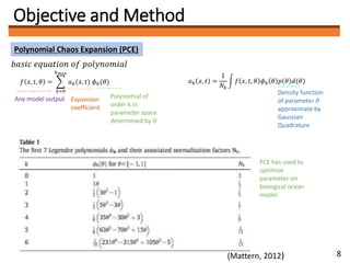
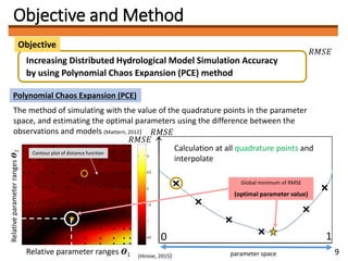
Downloaded 12 times
![Approach
In order to optimize the poorly known parameters and improve the model forecast
ability, data assimilation is required
Input and/or parameters
Uncertain characterisation
𝑥 = [𝑥1, 𝑥2, … … . . 𝑥 𝑛]
System simulation
• Process
• Equations
• Code
𝑦 = 𝑓(𝑥)
Outputs
𝑦 = [𝑦1, 𝑦2, … … . . 𝑦 𝑛]
- Parameter optimization
- Sensitivity analysis
- Distribution statistics
- Performance measures
(variance, RMSE)
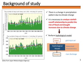
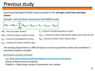
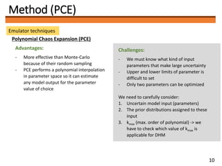
Characterization of uncertainty in hydrologic models is often critical for many water
resources applications (drought/ flood management, water supply utilities, reservoir
operation, sustainable water management, etc.).
4](https://image.slidesharecdn.com/cross-boundaryseminar-putika-2-180109033623/85/Improving-Distributed-Hydrologocal-Model-Simulation-Accuracy-Using-Polynomial-Chaos-Expansion-5-320.jpg)
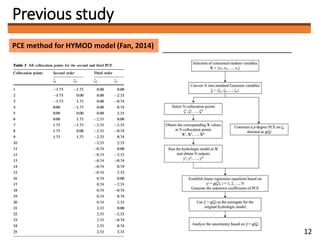
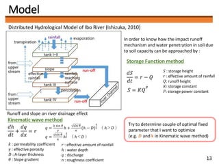
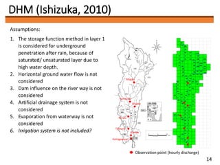
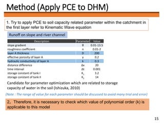
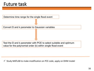

1) The document discusses applying the Polynomial Chaos Expansion (PCE) method to optimize parameters in distributed hydrological models and improve simulation accuracy. 2) PCE involves approximating a model output as a polynomial function of uncertain input parameters. It can efficiently estimate model outputs across the parameter space. 3) The author plans to use PCE to optimize soil-related parameters like layer thickness and hydraulic conductivity in a distributed hydrological model of the Ibo River catchment. Determining the optimal polynomial order for the model is a key future task.