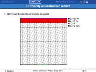
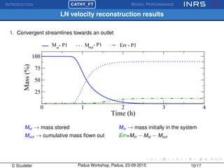
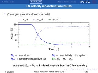
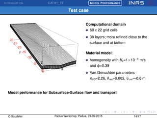
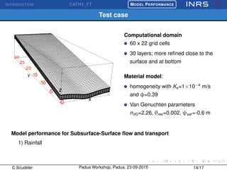
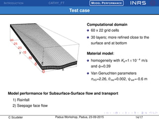
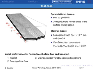
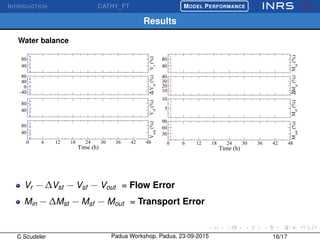
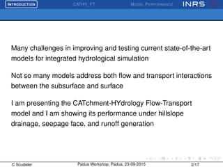
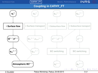
The document describes the CATchment-HYdrology Flow-Transport (CATHY_FT) model, which simulates coupled surface-subsurface flow and transport processes. CATHY_FT uses numerical models including the Richards' equation and advection-dispersion equation to simulate subsurface flow and transport, and finite difference schemes for surface processes. It features a sequential, explicit coupling between surface and subsurface calculations at each time step to account for interactions between domains. The presentation aims to demonstrate CATHY_FT's performance in simulating hydrological processes like hillslope drainage and runoff generation.

1. Hydrological modeling of coupled surface-subsurface
flow and transport phenomena: the
CATchment-HYdrology Flow-Transport (CATHY_FT)
model
Workshop on coupled hydrological modeling
Carlotta Scudeler, Claudio Paniconi, Mario Putti
Padua, 23-09-2015

2. £
¢
¡INTRODUCTION CATHY_FT MODEL PERFORMANCE
Many challenges in improving and testing current state-of-the-art
models for integrated hydrological simulation
Not so many models address both flow and transport interactions
between the subsurface and surface
I am presenting the CATchment-HYdrology Flow-Transport
model and I am showing its performance under hillslope
drainage, seepage face, and runoff generation
C Scudeler Padua Workshop, Padua, 23-09-2015 2/17

3. II. CATchment HYdrology Flow
and Transport model

4. INTRODUCTION
£
¢
¡CATHY_FT MODEL PERFORMANCE
CATchment HYdrology (CATHY) model



Sw Ss
∂ψ
∂t
+ φ∂Sw
∂t
= − · q + qss
∂Q
∂t
+ ck
∂Q
∂s
= Dh
∂2
Q
∂s2 + ck qs



∂θc
∂t
= · [−qc + D c] + qtss
∂Qm
∂t
+ ct
∂Qm
∂s
= Dc
∂2
Qm
∂s2 + ct qts
C Scudeler Padua Workshop, Padua, 23-09-2015 4/17

5. INTRODUCTION
£
¢
¡CATHY_FT MODEL PERFORMANCE
CATHY Flow-Transport (CATHY_FT) model



Sw Ss
∂ψ
∂t
+ φ∂Sw
∂t
= − · q + qss
∂Q
∂t
+ ck
∂Q
∂s
= Dh
∂2
Q
∂s2 + ck qs



∂θc
∂t
= · [−qc + D c] + qtss
∂Qm
∂t
+ ct
∂Qm
∂s
= Dc
∂2
Qm
∂s2 + ct qts
C Scudeler Padua Workshop, Padua, 23-09-2015 5/17

6. INTRODUCTION
£
¢
¡CATHY_FT MODEL PERFORMANCE
Numerical model
Richards’ equation (subsurface flow)



Sw Ss
∂ψ
∂t
+ φ∂Sw
∂t
= − · q + qss
∂Q
∂t
+ ck
∂Q
∂s
= Dh
∂2
Q
∂s2 + ck qs



∂θc
∂t
= · [−qc + D c] + qtss
∂Qm
∂t
+ ct
∂Qm
∂s
= Dc
∂2
Qm
∂s2 + ct qts
Numerics: P1 Galerkin finite element (FE) model in space and implicit finite difference
model in time
C Scudeler Padua Workshop, Padua, 23-09-2015 6/17

7. INTRODUCTION
£
¢
¡CATHY_FT MODEL PERFORMANCE
Numerical model
Richards’ equation (subsurface flow)



Sw Ss
∂ψ
∂t
+ φ∂Sw
∂t
= − · q + qss
∂Q
∂t
+ ck
∂Q
∂s
= Dh
∂2
Q
∂s2 + ck qs



∂θc
∂t
= · [−qc + D c] + qtss
∂Qm
∂t
+ ct
∂Qm
∂s
= Dc
∂2
Qm
∂s2 + ct qts
Numerics: P1 Galerkin finite element (FE) model in space and implicit finite difference
model in time
1. Nodal solution for ψ → continuous and piecewise linear
C Scudeler Padua Workshop, Padua, 23-09-2015 6/17

8. INTRODUCTION
£
¢
¡CATHY_FT MODEL PERFORMANCE
Numerical model
Richards’ equation (subsurface flow)



Sw Ss
∂ψ
∂t
+ φ∂Sw
∂t
= − · q + qss
∂Q
∂t
+ ck
∂Q
∂s
= Dh
∂2
Q
∂s2 + ck qs



∂θc
∂t
= · [−qc + D c] + qtss
∂Qm
∂t
+ ct
∂Qm
∂s
= Dc
∂2
Qm
∂s2 + ct qts
Numerics: P1 Galerkin finite element (FE) model in space and implicit finite difference
model in time
1. Nodal solution for ψ → continuous and piecewise linear
2. Elementwise post-computation of the velocity field q from direct application of
Darcy’s law → elementwise constant, normal flux discontinous and not
mass-conservative across every face
C Scudeler Padua Workshop, Padua, 23-09-2015 6/17

9. INTRODUCTION
£
¢
¡CATHY_FT MODEL PERFORMANCE
Numerical model
Richards’ equation (subsurface flow)



Sw Ss
∂ψ
∂t
+ φ∂Sw
∂t
= − · q + qss
∂Q
∂t
+ ck
∂Q
∂s
= Dh
∂2
Q
∂s2 + ck qs



∂θc
∂t
= · [−qc + D c] + qtss
∂Qm
∂t
+ ct
∂Qm
∂s
= Dc
∂2
Qm
∂s2 + ct qts
Numerics: P1 Galerkin finite element (FE) model in space and implicit finite difference
model in time
1. Nodal solution for ψ → continuous and piecewise linear
2. Elementwise post-computation of the velocity field q from direct application of
Darcy’s law → elementwise constant, normal flux discontinous and not
mass-conservative across every face
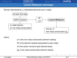
3. Larson-Niklasson (LN) velocity field q reconstruction
C Scudeler Padua Workshop, Padua, 23-09-2015 6/17

10. INTRODUCTION
£
¢
¡CATHY_FT MODEL PERFORMANCE
Numerical model
ADE equation (subsurface transport)



Sw Ss
∂ψ
∂t
+ φ∂Sw
∂t
= − · q + qss
∂Q
∂t
+ ck
∂Q
∂s
= Dh
∂2
Q
∂s2 + ck qs



∂θc
∂t
= · [−qc + D c] + qtss
∂Qm
∂t
+ ct
∂Qm
∂s
= Dc
∂2
Qm
∂s2 + ct qts
Numerics: High resolution finite volume (for - · qc advective step) and FE (for
· (D c) dispersive step) combined with a time-splitting technique
C Scudeler Padua Workshop, Padua, 23-09-2015 6/17

11. INTRODUCTION
£
¢
¡CATHY_FT MODEL PERFORMANCE
Numerical model
ADE equation (subsurface transport)



Sw Ss
∂ψ
∂t
+ φ∂Sw
∂t
= − · q + qss
∂Q
∂t
+ ck
∂Q
∂s
= Dh
∂2
Q
∂s2 + ck qs



∂θc
∂t
= · [−qc + D c] + qtss
∂Qm
∂t
+ ct
∂Qm
∂s
= Dc
∂2
Qm
∂s2 + ct qts
Numerics: High resolution finite volume (for - · qc advective step) and FE (for
· (D c) dispersive step) combined with a time-splitting technique
1. Advective time-explicit step for the elementwise c
C Scudeler Padua Workshop, Padua, 23-09-2015 6/17

12. INTRODUCTION
£
¢
¡CATHY_FT MODEL PERFORMANCE
Numerical model
ADE equation (subsurface transport)



Sw Ss
∂ψ
∂t
+ φ∂Sw
∂t
= − · q + qss
∂Q
∂t
+ ck
∂Q
∂s
= Dh
∂2
Q
∂s2 + ck qs



∂θc
∂t
= · [−qc + D c] + qtss
∂Qm
∂t
+ ct
∂Qm
∂s
= Dc
∂2
Qm
∂s2 + ct qts
Numerics: High resolution finite volume (for - · qc advective step) and FE (for
· (D c) dispersive step) combined with a time-splitting technique
1. Advective time-explicit step for the elementwise c
2. Mass-conservative element→node c reconstruction
C Scudeler Padua Workshop, Padua, 23-09-2015 6/17

13. INTRODUCTION
£
¢
¡CATHY_FT MODEL PERFORMANCE
Numerical model
ADE equation (subsurface transport)



Sw Ss
∂ψ
∂t
+ φ∂Sw
∂t
= − · q + qss
∂Q
∂t
+ ck
∂Q
∂s
= Dh
∂2
Q
∂s2 + ck qs



∂θc
∂t
= · [−qc + D c] + qtss
∂Qm
∂t
+ ct
∂Qm
∂s
= Dc
∂2
Qm
∂s2 + ct qts
Numerics: High resolution finite volume (for - · qc advective step) and FE (for
· (D c) dispersive step) combined with a time-splitting technique
1. Advective time-explicit step for the elementwise c
2. Mass-conservative element→node c reconstruction
3. Dispersive time-implicit step for the nodal c
C Scudeler Padua Workshop, Padua, 23-09-2015 6/17

14. INTRODUCTION
£
¢
¡CATHY_FT MODEL PERFORMANCE
Numerical model
ADE equation (subsurface transport)



Sw Ss
∂ψ
∂t
+ φ∂Sw
∂t
= − · q + qss
∂Q
∂t
+ ck
∂Q
∂s
= Dh
∂2
Q
∂s2 + ck qs



∂θc
∂t
= · [−qc + D c] + qtss
∂Qm
∂t
+ ct
∂Qm
∂s
= Dc
∂2
Qm
∂s2 + ct qts
Numerics: High resolution finite volume (for - · qc advective step) and FE (for
· (D c) dispersive step) combined with a time-splitting technique
1. Advective time-explicit step for the elementwise c
2. Mass-conservative element→node c reconstruction
3. Dispersive time-implicit step for the nodal c
4. Mass-conservative node→element c reconstruction
C Scudeler Padua Workshop, Padua, 23-09-2015 6/17

15. INTRODUCTION
£
¢
¡CATHY_FT MODEL PERFORMANCE
Numerical model
Surface flow and transport equations



Sw Ss
∂ψ
∂t
+ φ∂Sw
∂t
= − · q + qss
∂Q
∂t
+ ck
∂Q
∂s
= Dh
∂2
Q
∂s2 + ck qs



∂θc
∂t
= · [−qc + D c] + qtss
∂Qm
∂t
+ ct
∂Qm
∂s
= Dc
∂2
Qm
∂s2 + ct qts
Numerics: Explicit finite difference scheme in space and time for both surface flow and
transport solution
C Scudeler Padua Workshop, Padua, 23-09-2015 6/17

16. INTRODUCTION
£
¢
¡CATHY_FT MODEL PERFORMANCE
Coupling in CATHY_FT
1 Surface flow 2 Surface transport 3 Subsurface flow 4 Subsurface transport
qs
k
qts
k
Qk+1
,hk+1
Qm
k+1
,csurf
k+1
ψk+1
,qk+1
BC switching
ck+1
BC switchingqss
k+1
Atmospheric BCk+1
qss
k+1
qtss
k+1
qtss
k+1
qs
k+1
qts
k+1
C Scudeler Padua Workshop, Padua, 23-09-2015 7/17

17. INTRODUCTION
£
¢
¡CATHY_FT MODEL PERFORMANCE
Coupling in CATHY_FT
1 Surface flow 2 Surface transport 3 Subsurface flow 4 Subsurface transport
qs
k
qts
k
Qk+1
,hk+1
Qm
k+1
,csurf
k+1
ψk+1
,qk+1
BC switching
Atmospheric BCk+1
ck+1
BC switchingqss
k+1
qss
k+1
qtss
k+1
qtss
k+1
qs
k+1
qts
k+1
C Scudeler Padua Workshop, Padua, 23-09-2015 7/17

18. INTRODUCTION
£
¢
¡CATHY_FT MODEL PERFORMANCE
Coupling in CATHY_FT
1 Surface flow 2 Surface transport 3 Subsurface flow 4 Subsurface transport
qs
k
qts
k
Qk+1
,hk+1
Qm
k+1
,csurf
k+1
Atmospheric BCk+1
ψk+1
,qk+1
BC switching
ck+1
BC switchingqss
k+1
qss
k+1
qtss
k+1
qtss
k+1
qs
k+1
qts
k+1
C Scudeler Padua Workshop, Padua, 23-09-2015 7/17

19. INTRODUCTION
£
¢
¡CATHY_FT MODEL PERFORMANCE
Coupling in CATHY_FT
1 Surface flow 2 Surface transport 3 Subsurface flow 4 Subsurface transport
qs
k
qts
k
Qk+1
,hk+1
Atmospheric BCk+1
Qm
k+1
,csurf
k+1
ψk+1
,qk+1
BC switching
ck+1
BC switchingqss
k+1
qss
k+1
qtss
k+1
qtss
k+1
qs
k+1
qts
k+1
C Scudeler Padua Workshop, Padua, 23-09-2015 7/17

20. INTRODUCTION
£
¢
¡CATHY_FT MODEL PERFORMANCE
Coupling in CATHY_FT
1 Surface flow 2 Surface transport 3 Subsurface flow
Atmospheric BCk+1
4 Subsurface transport
qs
k
qts
k
Qk+1
,hk+1
Qm
k+1
,csurf
k+1
ψk+1
,qk+1
BC switching
ck+1
BC switchingqss
k+1
qss
k+1
qtss
k+1
qtss
k+1
qs
k+1
qts
k+1
C Scudeler Padua Workshop, Padua, 23-09-2015 7/17

21. INTRODUCTION
£
¢
¡CATHY_FT MODEL PERFORMANCE
Model accuracy
Ability of the model to conserve mass
C Scudeler Padua Workshop, Padua, 23-09-2015 8/17

22. INTRODUCTION
£
¢
¡CATHY_FT MODEL PERFORMANCE
Model accuracy
Ability of the model to conserve mass
Sw Ss
∂ψ
∂t
+ φ
∂Sw
∂t
= − · q + qss
→
Mass-conservative solution
achieved solving the equation in
its ψ − Sw mixed form [Celia et al.,
1990]
C Scudeler Padua Workshop, Padua, 23-09-2015 8/17

23. INTRODUCTION
£
¢
¡CATHY_FT MODEL PERFORMANCE
Model accuracy
Ability of the model to conserve mass
∂θc
∂t
= · [−qc + D c] + qtss
→
HRFV mass-conservative solution
if q is mass-conservative.
C Scudeler Padua Workshop, Padua, 23-09-2015 8/17

24. INTRODUCTION
£
¢
¡CATHY_FT MODEL PERFORMANCE
Model accuracy
Ability of the model to conserve mass
∂θc
∂t
= · [−qc + D c] + qtss
→
HRFV mass-conservative solution
if q is mass-conservative.
P1 Galerkin q is not
mass-conservative
C Scudeler Padua Workshop, Padua, 23-09-2015 8/17

25. INTRODUCTION
£
¢
¡CATHY_FT MODEL PERFORMANCE
Model accuracy
Ability of the model to conserve mass
∂θc
∂t
= · [−qc + D c] + qtss
→
HRFV mass-conservative solution
if q is mass-conservative.
P1 Galerkin q is not
mass-conservative
To make q mass-conservative:
change the numerical scheme from FE =⇒ High computational cost
to Mixed Hybrid Finite Element (MHFE)
or
add mass-conservative velocity field =⇒ Low computational cost
reconstruction
C Scudeler Padua Workshop, Padua, 23-09-2015 8/17

26. INTRODUCTION
£
¢
¡CATHY_FT MODEL PERFORMANCE
Model accuracy
Ability of the model to conserve mass
∂θc
∂t
= · [−qc + D c] + qtss
→
HRFV mass-conservative solution
if q is mass-conservative.
P1 Galerkin q is not
mass-conservative
To make q mass-conservative:
change the numerical scheme from FE =⇒ High computational cost
to Mixed Hybrid Finite Element (MHFE)
or
add mass-conservative velocity field =⇒ Low computational cost
reconstruction
In CATHY_FT: FE =⇒ FE+Larson-Niklasson (LN) post-processing technique
C Scudeler Padua Workshop, Padua, 23-09-2015 8/17

27. INTRODUCTION
£
¢
¡CATHY_FT MODEL PERFORMANCE
Larson-Niklasson technique
Domain discretized by ne tetrahedral elements and n nodes
At each time step
C Scudeler Padua Workshop, Padua, 23-09-2015 9/17

28. INTRODUCTION
£
¢
¡CATHY_FT MODEL PERFORMANCE
Larson-Niklasson technique
Domain discretized by ne tetrahedral elements and n nodes
At each time step
CATHY solution
· ψ nodal solution
· qe
non mass-conservative
where:
qe
is the non mass-conservative element velocity
C Scudeler Padua Workshop, Padua, 23-09-2015 9/17

29. INTRODUCTION
£
¢
¡CATHY_FT MODEL PERFORMANCE
Larson-Niklasson technique
Domain discretized by ne tetrahedral elements and n nodes
At each time step
CATHY solution
· ψ nodal solution
· qe
non mass-conservative
· Re
i
· q·n
where:
qe
is the non mass-conservative element velocity
Re
i is the element residual associated to each node i
n is the vector normal to each element faces
C Scudeler Padua Workshop, Padua, 23-09-2015 9/17

30. INTRODUCTION
£
¢
¡CATHY_FT MODEL PERFORMANCE
Larson-Niklasson technique
Domain discretized by ne tetrahedral elements and n nodes
At each time step
CATHY solution
· ψ nodal solution
· qe
non mass-conservative
· Re
i
· q·n
Larson-Niklasson
· new qLN ·n
· new mass-conservative qe
LN
where:
qe
is the non mass-conservative element velocity
Re
i is the element residual associated to each node i
n is the vector normal to each element faces
qe
LN is the mass-conservative element velocity
C Scudeler Padua Workshop, Padua, 23-09-2015 9/17

31. INTRODUCTION
£
¢
¡CATHY_FT MODEL PERFORMANCE
LN velocity reconstruction results
1. Convergent streamlines towards an outlet
2. High streamline curvatures due to heterogeneity
C Scudeler Padua Workshop, Padua, 23-09-2015 10/17

32. INTRODUCTION
£
¢
¡CATHY_FT MODEL PERFORMANCE
LN velocity reconstruction results
1. Convergent streamlines towards an outlet
D=50 m
D=0 m
qN=0 m/s
cin =1
C Scudeler Padua Workshop, Padua, 23-09-2015 10/17

33. INTRODUCTION
£
¢
¡CATHY_FT MODEL PERFORMANCE
LN velocity reconstruction results
1. Convergent streamlines towards an outlet
0 1 2 3 4
Time (h)
25
50
75
100
Mass(%)
Mst
- P1 Mout
- P1 Err - P1
Mst → mass stored
Mout → cumulative mass flown out
Min → mass initially in the system
Err=Min − Mst − Mout
C Scudeler Padua Workshop, Padua, 23-09-2015 10/17

34. INTRODUCTION
£
¢
¡CATHY_FT MODEL PERFORMANCE
LN velocity reconstruction results
1. Convergent streamlines towards an outlet
0 1 2 3 4
Time (h)
25
50
75
100
Mass(%)
Mst
- P1 Mout
- P1 Err - P1
Mst → mass stored
Mout → cumulative mass flown out
Min → mass initially in the system
Err=Min − Mst − Mout
At the end Mout = Min ⇒ P1 Galerkin q exits from the 0 flux boundary
C Scudeler Padua Workshop, Padua, 23-09-2015 10/17

35. INTRODUCTION
£
¢
¡CATHY_FT MODEL PERFORMANCE
LN velocity reconstruction results
1. Convergent streamlines towards an outlet
0 1 2 3 4
Time (h)
25
50
75
100
Mass(%)
Mst
- LN Mout
- LN
C Scudeler Padua Workshop, Padua, 23-09-2015 10/17

36. INTRODUCTION
£
¢
¡CATHY_FT MODEL PERFORMANCE
LN velocity reconstruction results
1. Convergent streamlines towards an outlet
0 1 2 3 4
Time (h)
25
50
75
100
Mass(%)
Mst
- LN Mout
- LN
Velocities reconstructed with LN do not violate the 0 flux boundaries
C Scudeler Padua Workshop, Padua, 23-09-2015 10/17

37. INTRODUCTION
£
¢
¡CATHY_FT MODEL PERFORMANCE
LN velocity reconstruction results
1. Convergent streamlines towards an outlet
2. High streamline curvatures due to heterogeneity
D=50 m
D=0 m
qN=0 m/s
cin =1
Ks (m/s)
2x10-4
2x10-12
C Scudeler Padua Workshop, Padua, 23-09-2015 11/17

38. INTRODUCTION
£
¢
¡CATHY_FT MODEL PERFORMANCE
LN velocity reconstruction results
1. Convergent streamlines towards an outlet
2. High streamline curvatures due to heterogeneity
0 2 4 6 8 10
Time (h)
Mst
- LN Mstf
- LN
0 2 4 6 8
Time (h)
25
50
75
100
Mass(%)
Mst
- P1 Mstf
- P1
Mstf
→ mass stored in the unpermeable soil Mst → mass stored
C Scudeler Padua Workshop, Padua, 23-09-2015 11/17

39. INTRODUCTION
£
¢
¡CATHY_FT MODEL PERFORMANCE
LN velocity reconstruction results
1. Convergent streamlines towards an outlet
2. High streamline curvatures due to heterogeneity
0 2 4 6 8 10
Time (h)
Mst
- LN Mstf
- LN
0 2 4 6 8
Time (h)
25
50
75
100
Mass(%)
Mst
- P1 Mstf
- P1
Mstf
→ mass stored in the unpermeable soil Mst → mass stored
At the end for P1 Mstf
= Mst =0 ⇒ Solute mass get trapped in the unpermeable soil
At the end for LN Mstf
= Mst =0 ⇒ Solute mass slightly crosses the unpermeable soil
C Scudeler Padua Workshop, Padua, 23-09-2015 11/17

40. III. Testing CATHY_FT at the
Landscape Evolution
Observatory (LEO)

41. INTRODUCTION CATHY_FT
£
¢
¡MODEL PERFORMANCE
The Landscape Evolution Observatory (LEO)
LEO, Biosphere 2, Oracle,
Arizona, U.S.A.
3 convergent landscapes
30 m long, 11.5 m wide
dense sensor and sampler
network
rainfall simulator (3-45
mm/h)
C Scudeler Padua Workshop, Padua, 23-09-2015 13/17

42. INTRODUCTION CATHY_FT
£
¢
¡MODEL PERFORMANCE
The Landscape Evolution Observatory (LEO)
LEO, Biosphere 2, Oracle,
Arizona, U.S.A.
3 convergent landscapes
30 m long, 11.5 m wide
dense sensor and sampler
network
rainfall simulator (3-45
mm/h)
In Figure:
View of one of the three
hillslopes from top
C Scudeler Padua Workshop, Padua, 23-09-2015 13/17

43. INTRODUCTION CATHY_FT
£
¢
¡MODEL PERFORMANCE
The Landscape Evolution Observatory (LEO)
LEO, Biosphere 2, Oracle,
Arizona, U.S.A.
3 convergent landscapes
30 m long, 11.5 m wide
dense sensor and sampler
network
rainfall simulator (3-45
mm/h)
In Figure:
View of one of the three
hillslopes from top
Tipping bucket for low seepage
face flow
C Scudeler Padua Workshop, Padua, 23-09-2015 13/17

44. INTRODUCTION CATHY_FT
£
¢
¡MODEL PERFORMANCE
The Landscape Evolution Observatory (LEO)
LEO, Biosphere 2, Oracle,
Arizona, U.S.A.
3 convergent landscapes
30 m long, 11.5 m wide
dense sensor and sampler
network
rainfall simulator (3-45
mm/h)
In Figure:
View of one of the three
hillslopes from top
Tipping bucket for low seepage
face flow
Rainfall simulator
C Scudeler Padua Workshop, Padua, 23-09-2015 13/17

45. INTRODUCTION CATHY_FT
£
¢
¡MODEL PERFORMANCE
Test case
Computational domain
60 x 22 grid cells
30 layers; more refined close to the
surface and at bottom
C Scudeler Padua Workshop, Padua, 23-09-2015 14/17

46. INTRODUCTION CATHY_FT
£
¢
¡MODEL PERFORMANCE
Test case
Computational domain
60 x 22 grid cells
30 layers; more refined close to the
surface and at bottom
Material model:
homogeneity with Ks=1×10−4
m/s
and φ=0.39
Van Genuchten parameters
nVG=2.26, θres=0.002, ψsat =-0.6 m
C Scudeler Padua Workshop, Padua, 23-09-2015 14/17

47. INTRODUCTION CATHY_FT
£
¢
¡MODEL PERFORMANCE
Test case
Computational domain
60 x 22 grid cells
30 layers; more refined close to the
surface and at bottom
Material model:
homogeneity with Ks=1×10−4
m/s
and φ=0.39
Van Genuchten parameters
nVG=2.26, θres=0.002, ψsat =-0.6 m
Model performance for Subsurface-Surface flow and transport
C Scudeler Padua Workshop, Padua, 23-09-2015 14/17

48. INTRODUCTION CATHY_FT
£
¢
¡MODEL PERFORMANCE
Test case
Computational domain
60 x 22 grid cells
30 layers; more refined close to the
surface and at bottom
Material model:
homogeneity with Ks=1×10−4
m/s
and φ=0.39
Van Genuchten parameters
nVG=2.26, θres=0.002, ψsat =-0.6 m
Model performance for Subsurface-Surface flow and transport
1) Rainfall
C Scudeler Padua Workshop, Padua, 23-09-2015 14/17

49. INTRODUCTION CATHY_FT
£
¢
¡MODEL PERFORMANCE
Test case
Computational domain
60 x 22 grid cells
30 layers; more refined close to the
surface and at bottom
Material model:
homogeneity with Ks=1×10−4
m/s
and φ=0.39
Van Genuchten parameters
nVG=2.26, θres=0.002, ψsat =-0.6 m
Model performance for Subsurface-Surface flow and transport
1) Rainfall
2) Seepage face flow
C Scudeler Padua Workshop, Padua, 23-09-2015 14/17

50. INTRODUCTION CATHY_FT
£
¢
¡MODEL PERFORMANCE
Test case
Computational domain
60 x 22 grid cells
30 layers; more refined close to the
surface and at bottom
Material model:
homogeneity with Ks=1×10−4
m/s
and φ=0.39
Van Genuchten parameters
nVG=2.26, θres=0.002, ψsat =-0.6 m
Model performance for Subsurface-Surface flow and transport
1) Rainfall
2) Seepage face flow
3) Drainage under variably saturated conditions
C Scudeler Padua Workshop, Padua, 23-09-2015 14/17

51. INTRODUCTION CATHY_FT
£
¢
¡MODEL PERFORMANCE
Test case
Computational domain
60 x 22 grid cells
30 layers; more refined close to the
surface and at bottom
Material model:
homogeneity with Ks=1×10−4
m/s
and φ=0.39
Van Genuchten parameters
nVG=2.26, θres=0.002, ψsat =-0.6 m
Model performance for Subsurface-Surface flow and transport
1) Rainfall
2) Seepage face flow
3) Drainage under variably saturated conditions
4) Surface flow
C Scudeler Padua Workshop, Padua, 23-09-2015 14/17

52. INTRODUCTION CATHY_FT
£
¢
¡MODEL PERFORMANCE
Test case
Seepage Face
Outlet
Computational domain
60 x 22 grid cells
30 layers; more refined close to the
surface and at bottom
Material model:
homogeneity with Ks=1×10−4
m/s
and φ=0.39
Van Genuchten parameters
nVG=2.26, θres=0.002, ψsat =-0.6 m
Model performance for Subsurface-Surface flow and transport
1) Rainfall
2) Seepage face flow
3) Drainage under variably saturated conditions
4) Surface flow
C Scudeler Padua Workshop, Padua, 23-09-2015 14/17

53. INTRODUCTION CATHY_FT
£
¢
¡MODEL PERFORMANCE
Input
Water and solute mass inflow Cumulative volume and mass
0.005
0.01
0.015
Qr
(m
3
/s)
0 6 12 18 24 30 36 42 48
Time (h)
0.005
0.01
0.015
Qm
(mg/s)
15
30
45
60
Vr
(m
3
)
0 6 12 18 24 30 36 42 48
Time (h)
15
30
45
60
Min
(mg)
Initial conditions: 119 m3
of water initially present in the system (water table set at 0.4 m
from bottom) and 0 solute mass
C Scudeler Padua Workshop, Padua, 23-09-2015 15/17

54. INTRODUCTION CATHY_FT
£
¢
¡MODEL PERFORMANCE
Input
Water and solute mass inflow Cumulative volume and mass
0.005
0.01
0.015
Qr
(m
3
/s)
0 6 12 18 24 30 36 42 48
Time (h)
0.005
0.01
0.015
Qm
(mg/s)
Qr=0.012 m3
/s
15
30
45
60
Vr
(m
3
)
0 6 12 18 24 30 36 42 48
Time (h)
15
30
45
60
Min
(mg)
Vr=40.4 m3
Initial conditions: 119 m3
of water initially present in the system (water table set at 0.4 m
from bottom) and 0 solute mass
Flow input: pulse of homogenous rain Qr =0.012 m3
/s for 1 h→ cumulative volume
injected Vr =40.4 m3
C Scudeler Padua Workshop, Padua, 23-09-2015 15/17

55. INTRODUCTION CATHY_FT
£
¢
¡MODEL PERFORMANCE
Input
Water and solute mass inflow Cumulative volume and mass
0.005
0.01
0.015
Qr
(m
3
/s)
0 6 12 18 24 30 36 42 48
Time (h)
0.005
0.01
0.015
Qm
(mg/s)
Qm=0.012 mg/s
15
30
45
60
Vr
(m
3
)
0 6 12 18 24 30 36 42 48
Time (h)
15
30
45
60
Min
(mg)
Min=40.4 mg
Initial conditions: 119 m3
of water initially present in the system (water table set at 0.4 m
from bottom) and 0 solute mass
Flow input: pulse of homogenous rain Qr =0.012 m3
/s for 1 h→ cumulative volume
injected Vr =40.4 m3
Transport input: solute injection with c=1 mg/m3
of rain pulse→ mass inflow Qm=0.012
mg/s and cumulative mass injected Min=40.4 mg
C Scudeler Padua Workshop, Padua, 23-09-2015 15/17

56. INTRODUCTION CATHY_FT
£
¢
¡MODEL PERFORMANCE
Results
Water balance
40
80
Vr
(%)
-40
0
40
80
∆Vst
(%)
40
80
Vsf
(%)
0 6 12 18 24 30 36 42 48
Time (h)
40
80
Vout
(%)
40
80
Min
(%)
10
20
30
40
∆Mst
(%)
5
10
Msf
(%)
0 6 12 18 24 30 36 42 48
Time (h)
30
60
90
Mout
(%)
Vr − ∆Vst − Vsf − Vout = Flow Error
Min − ∆Mst − Msf − Mout = Transport Error
C Scudeler Padua Workshop, Padua, 23-09-2015 16/17

57. INTRODUCTION CATHY_FT
£
¢
¡MODEL PERFORMANCE
Results
Water balance
40
80
Vr
(%)
-40
0
40
80
∆Vst
(%)
40
80
Vsf
(%)
0 6 12 18 24 30 36 42 48
Time (h)
40
80
Vout
(%)
Vr=100%
40
80
Min
(%)
10
20
30
40
∆Mst
(%)
5
10
Msf
(%)
0 6 12 18 24 30 36 42 48
Time (h)
30
60
90
Mout
(%)
Vr − ∆Vst − Vsf − Vout ⇒100
Min − ∆Mst − Msf − Mout = Transport Error
C Scudeler Padua Workshop, Padua, 23-09-2015 16/17

58. INTRODUCTION CATHY_FT
£
¢
¡MODEL PERFORMANCE
Results
Water balance
40
80
Vr
(%)
-40
0
40
80
∆Vst
(%)
40
80
Vsf
(%)
0 6 12 18 24 30 36 42 48
Time (h)
40
80
Vout
(%)
-48.17%∆Vst=
40
80
Min
(%)
10
20
30
40
∆Mst
(%)
5
10
Msf
(%)
0 6 12 18 24 30 36 42 48
Time (h)
30
60
90
Mout
(%)
Vr − ∆Vst − Vsf − Vout ⇒100+48.17
Min − ∆Mst − Msf − Mout = Transport Error
C Scudeler Padua Workshop, Padua, 23-09-2015 16/17

59. INTRODUCTION CATHY_FT
£
¢
¡MODEL PERFORMANCE
Results
Water balance
40
80
Vr
(%)
-40
0
40
80
∆Vst
(%)
40
80
Vsf
(%)
0 6 12 18 24 30 36 42 48
Time (h)
40
80
Vout
(%)
Vsf=77.62%
40
80
Min
(%)
10
20
30
40
∆Mst
(%)
5
10
Msf
(%)
0 6 12 18 24 30 36 42 48
Time (h)
30
60
90
Mout
(%)
Vr − ∆Vst − Vsf − Vout ⇒100+48.17-77.62
Min − ∆Mst − Msf − Mout = Transport Error
C Scudeler Padua Workshop, Padua, 23-09-2015 16/17

60. INTRODUCTION CATHY_FT
£
¢
¡MODEL PERFORMANCE
Results
Water balance
40
80
Vr
(%)
-40
0
40
80
∆Vst
(%)
40
80
Vsf
(%)
0 6 12 18 24 30 36 42 48
Time (h)
40
80
Vout
(%)
Vout=70.58%
40
80
Min
(%)
10
20
30
40
∆Mst
(%)
5
10
Msf
(%)
0 6 12 18 24 30 36 42 48
Time (h)
30
60
90
Mout
(%)
Vr − ∆Vst − Vsf − Vout ⇒100+48.17-77.62-70.58=o(0.01)%
Min − ∆Mst − Msf − Mout = Transport Error
C Scudeler Padua Workshop, Padua, 23-09-2015 16/17

61. INTRODUCTION CATHY_FT
£
¢
¡MODEL PERFORMANCE
Results
Mass balance
40
80
Vr
(%)
-40
0
40
80
∆Vst
(%)
40
80
Vsf
(%)
0 6 12 18 24 30 36 42 48
Time (h)
40
80
Vout
(%)
40
80
Min
(%)
10
20
30
40
∆Mst
(%)
5
10
Msf
(%)
0 6 12 18 24 30 36 42 48
Time (h)
30
60
90
Mout
(%)
Min=100%
Vr − ∆Vst − Vsf − Vout ⇒100+48.17-77.62-70.58=o(0.01)%
Min − ∆Mst − Msf − Mout ⇒100
C Scudeler Padua Workshop, Padua, 23-09-2015 16/17

62. INTRODUCTION CATHY_FT
£
¢
¡MODEL PERFORMANCE
Results
Mass balance
40
80
Vr
(%)
-40
0
40
80
∆Vst
(%)
40
80
Vsf
(%)
0 6 12 18 24 30 36 42 48
Time (h)
40
80
Vout
(%)
40
80
Min
(%)
10
20
30
40
∆Mst
(%)
5
10
Msf
(%)
0 6 12 18 24 30 36 42 48
Time (h)
30
60
90
Mout
(%)
∆Mst=28.62%
Vr − ∆Vst − Vsf − Vout ⇒100+48.17-77.62-70.58=o(0.01)%
Min − ∆Mst − Msf − Mout ⇒100-28.62
C Scudeler Padua Workshop, Padua, 23-09-2015 16/17

63. INTRODUCTION CATHY_FT
£
¢
¡MODEL PERFORMANCE
Results
Mass balance
40
80
Vr
(%)
-40
0
40
80
∆Vst
(%)
40
80
Vsf
(%)
0 6 12 18 24 30 36 42 48
Time (h)
40
80
Vout
(%)
40
80
Min
(%)
10
20
30
40
∆Mst
(%)
5
10
Msf
(%)
0 6 12 18 24 30 36 42 48
Time (h)
30
60
90
Mout
(%)
Msf=6.86%
Vr − ∆Vst − Vsf − Vout ⇒100+48.17-77.62-70.58=o(0.01)%
Min − ∆Mst − Msf − Mout ⇒100-28.62-6.86
C Scudeler Padua Workshop, Padua, 23-09-2015 16/17

64. INTRODUCTION CATHY_FT
£
¢
¡MODEL PERFORMANCE
Results
Mass balance
40
80
Vr
(%)
-40
0
40
80
∆Vst
(%)
40
80
Vsf
(%)
0 6 12 18 24 30 36 42 48
Time (h)
40
80
Vout
(%)
40
80
Min
(%)
10
20
30
40
∆Mst
(%)
5
10
Msf
(%)
0 6 12 18 24 30 36 42 48
Time (h)
30
60
90
Mout
(%)
Mout=64.42%
Vr − ∆Vst − Vsf − Vout ⇒100+48.17-77.62-70.58=o(0.01)%
Min − ∆Mst − Msf − Mout ⇒100-28.62-6.86-64.42=o(0.1)%
C Scudeler Padua Workshop, Padua, 23-09-2015 16/17

65. INTRODUCTION CATHY_FT MODEL PERFORMANCE
Conclusions
1. P1 Galerkin solution is mass-conservative while the velocities are
not; this causes problems for transport simulations. This requires a
post-processing technique to ensure mass-conservation
C Scudeler Padua Workshop, Padua, 23-09-2015 17/17

66. INTRODUCTION CATHY_FT MODEL PERFORMANCE
Conclusions
1. P1 Galerkin solution is mass-conservative while the velocities are
not; this causes problems for transport simulations. This requires a
post-processing technique to ensure mass-conservation
2. Results so far indicate that LN reconstructed velocities are as
accurate as MHFE velocities and achieve much better computational
efficiency
C Scudeler Padua Workshop, Padua, 23-09-2015 17/17

67. INTRODUCTION CATHY_FT MODEL PERFORMANCE
Conclusions
1. P1 Galerkin solution is mass-conservative while the velocities are
not; this causes problems for transport simulations. This requires a
post-processing technique to ensure mass-conservation
2. Results so far indicate that LN reconstructed velocities are as
accurate as MHFE velocities and achieve much better computational
efficiency
3. Exchange processes in integrated surface-subsurface models are
highly complex and need to be carefully formulated and resolved
C Scudeler Padua Workshop, Padua, 23-09-2015 17/17

68. Thanks for your attention