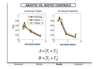
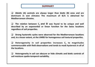
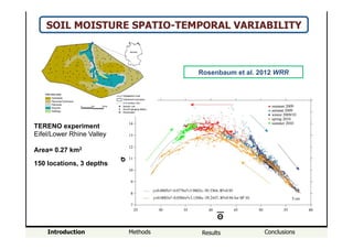
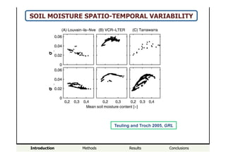
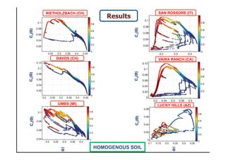
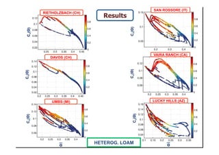
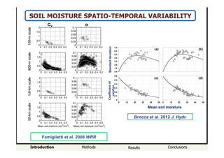
- Abiotic controls, like precipitation and evaporation, dominate soil moisture spatiotemporal variability in wet climates, while biotic controls from vegetation become more important in Mediterranean climates. - The relationship between the coefficient of variation (Cv) and mean soil moisture (Θ) was found to be unique and well described by an exponential or linear function for locations in Switzerland, but strong hysteretic cycles were observed for Mediterranean locations. 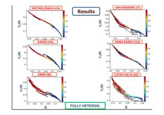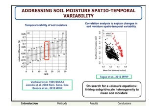- Heterogeneity in soil properties increases Cv and tends to obscure any hysteresis, masking climatic and biotic controls on soil moisture variability. Heterogeneity can therefore hide the influences of climate and vegetation on soil moisture spatiotemporal patterns.

1. Soil moisture spatio-temporal variability:
insights from mechanistic ecohydrological
modeling
Simone Fatichi
Institute of Environmental Engineering, ETH Zurich, Zurich, Switzerland
simone.fatichi@ifu.baug.ethz.ch
24 September 2015
Padova, Italy

2. Introduction Methods Results Conclusions
MOTIVATION
KNOWLEDGE of SOIL MOISTURE SPATIO-TEMPORAL VARIABILITY is
essential in a series of fields.
Remote sensing products of near surface soil moisture are becoming
widely available but they provide only an average value within a
footprint, while soil moisture is highly heterogeneous in space.
Ground based soil moisture sensors cannot be placed everywhere
EcologyMeteorologyHydrology

3. Introduction Methods Results Conclusions
ADDRESSING SOIL MOISTURE SPATIO-TEMPORAL
VARIABILITY
Tague et al., 2010 WRR
Vachaud et al. 1985 SSSAJ
Jacobs et al. 2004 Rem. Sens. Env.
Brocca et al., 2010 WRR
Temporal stability of soil moisture
Correlation analysis to explain changes in
soil moisture spatio-temporal variability
On search for a «closure equation»:
linking subgrid-scale heterogeneity to
mean soil moisture

4. Introduction Methods Results Conclusions
SOIL MOISTURE SPATIO-TEMPORAL VARIABILITY
10
15
20
10
15
20
25
30
35
11
12
13
14
15
Effective Saturation
0.6
0.7
0.8
10
15
20
10
15
20
25
30
35
11
12
13
14
15
Effective Saturation
0.6
0.7
0.8
Same mean ​" but different spatial variability Cv
Θ
Cv(Θ)
Effective Saturation Effective Saturation
t=1 t=2
t=3
Spatial coefficient of
variation!
t=4t=5
Mean soil moisture!

5. Introduction Methods Results Conclusions
Ivanov et al. 2010 WRR
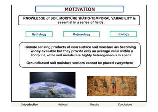
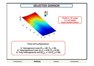
SOIL MOISTURE SPATIO-TEMPORAL VARIABILITY
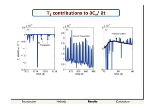
• Precipitation decreases
variability.
• Lateral re-distribution of
water increases variability
• ET drying decrease
variability
Lateral redistribution is
function of precipitation
intensity and pre-event soil
moisture (dependent on ET
history)
Mean domain soil moisture content [-]
Coefficientofvariation
tRIBS-VEGGIE

6. Introduction Methods Results Conclusions
SOIL MOISTURE SPATIO-TEMPORAL VARIABILITY
Famiglietti et al. 2008 WRR
Brocca et al. 2012 J. Hydr.
CV! σ!
Mean soil moisture
Coefficientof
varation
Standarddeviation

7. Introduction Methods Results Conclusions
SOIL MOISTURE SPATIO-TEMPORAL VARIABILITY
Rosenbaum et al. 2012 WRR
σ!
Θ
TERENO experiment
Eifel/Lower Rhine Valley
Area= 0.27 km2
150 locations, 3 depths

8. Introduction Methods Results Conclusions
SOIL MOISTURE SPATIO-TEMPORAL VARIABILITY
Teuling and Troch 2005, GRL
σ!σ!

9. Introduction Methods Results Conclusions
RESEARCH QUESTIONS
! (i) What is the relative importance of biotic and abiotic controls on
soil moisture spatio-temporal variability at the hillslope scale and
across different environmental conditions?
! (ii) Under what conditions is the relation between Cv and Θ
hysteretic or unique?

10. Introduction Methods Results Conclusions
METHOD: MECHANISTIC ECOHYDROLOGICAL MODEL
Tethys-Chloris
(T&C)
Explicit modeling of
shortwave and longwave
radiation through the
canopies
Energy budget solution,
with computation of
transpiration and
evaporation (resistance
analogy)
Hydrological Part
Biochemical model of
photosynthesis and
stomatal aperture
Fatichietal.,2012a,bJAMES,Fatichi2010
Snow hydrology component
(canopy interception, snow
density)

11. Introduction Methods Results Conclusions
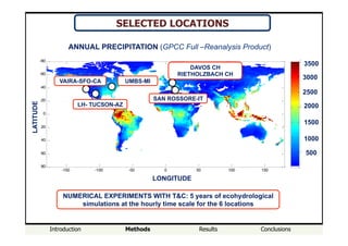
Domain spatial connectivity
RESOLUTION
5 to 100 [m]
• LATERAL CONNECTIONS BETWEEN
ELEMENTS (above surface and subsurface);
1D-quasi 3D approach
• SUBGRID PARAMETERIZATION FOR
CHANNELS
• KINEMATIC ROUTING (channel, subsurface,
overland)
TETHYS-CHLORIS (T&C)
Parallel version
Using distributed
computing resources

12. Introduction Methods Results Conclusions
Net Primary
productivity and plant
respiration
Carbon allocation and
translocation
Tissue turnover and
stress induced foliage
loss
Carbon balance on
different compartments
of the plant
Vegetation Component
Vegetation phenology
TETHYS-CHLORIS (T&C)
Fatichi et al., 2012a,b, J. Advances in Modeling Earth Systems
Fatichi and Leuzinger 2013, Agr. For. Met.
Fatichi et al., 2014, 2015 WRR,
Fatichi and Ivanov 2014, WRR
Pappas et al., 2015 NP; Paschalis et al., 2015, JGR

13. Introduction Methods Results Conclusions
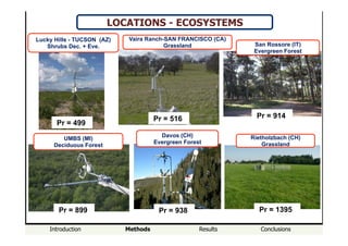
MODEL BENCHMARK
0 60 120 180
0
60
120
180
240
300
Time (min)
OutflowRate(m3
/min)
CATHY (sheet flow)
CATHY (comb. flow)
CATHY (rill flow)
Parflow
T&C
tRIBS
0 500 1000 1500 2000 0
500
1000
0
50
100
Y [m]
X [m]
Z[m]
Flow routing
(V-catchment domain)
Di Giammarco et al. 1996 J HYDR
Kollet and Maxwell, 2006, AWR
Panday and Huyakom 2004, AWR
Sulis et al. 2010, WRR
CATHY
(Camporese et al.
2010 WRR; Sulis et
al. 2010, WRR)
PARFLOW
(Kollet and Maxwell
2006, AWR; Maxwell
and Kollet 2008 Nat.
Geo.)
Integrated Hydrologic
Model Intercomparison
Workshop (Maxwell et
al. 2014, WRR)

14. Introduction Methods Results Conclusions
MODEL BENCHMARK
Integrated Hydrologic
Model Intercomparison
Workshop (Maxwell et al.
2014, WRR)
Anagnostopoulous et al. 2015, WRR
Sloping plane with
heterogeneous soil slab

15. Introduction Methods Results Conclusions
MODEL BENCHMARK
Generating runoff and trench flow in
an elementary hillslope (Biosphere-2
domain, Hopp et al., 2009 HESS).
HYDRUS-3D (Simunek et al., 2006; 2008)
tRIBS-VEGGIE (Ivanov et al., 2004; 2008 WRR)
0 100 200 300 400
0.1
0.15
0.2
0.25
0.3
0.35
WaterContentθ[-]
Hours
T&C
tRIBS-VEGGIE
HYDRUS-3D
0 100 200 300 400
0
0.5
1
1.5
2
TotalOutflow[m3
h-1
]
Hours
T&C
tRIBS-VEGGIE
HYDRUS-3D
Hopp et al. 2015, Hydr. Res. Sub.

16. Introduction Methods Results Conclusions
SELECTED DOMAIN
10
15
20
10
15
20
25
30
35
11
12
13
14
15
11
12
13
14
15
15x30 m 10° slope
1 m soil depth
Impermeable bottom
Three soil configurations:
1) Homogenous Loam (Psan =40 Pcla = 20)
2) Heterogeneous Loam (σlogKs = 0.28 Cv,Ks=0.29)
3) Fully heterogeneous soil (σlogKs = 1.23 Cv,Ks=1.08)

17. Introduction Methods Results Conclusions
-150 -100 -50 0 50 100 150
-80
-60
-40
-20
0
20
40
60
80
500
1000
1500
2000
2500
3000
3500
SELECTED LOCATIONS
ANNUAL PRECIPITATION (GPCC Full –Reanalysis Product)
3500
2000
1500
1000
500
VAIRA-SFO-CA UMBS-MI
LH- TUCSON-AZ
DAVOS CH
RIETHOLZBACH CH
LONGITUDE
LATITUDE
3000
2500
SAN ROSSORE-IT
NUMERICAL EXPERIMENTS WITH T&C: 5 years of ecohydrological
simulations at the hourly time scale for the 6 locations

18. Introduction Methods Results Conclusions
LOCATIONS - ECOSYSTEMS
Pr = 499!
Vaira Ranch-SAN FRANCISCO (CA)
Grassland
UMBS (MI)
Deciduous Forest
Lucky Hills - TUCSON (AZ)
Shrubs Dec. + Eve.
Rietholzbach (CH)
Grassland
Davos (CH)
Evergreen Forest
San Rossore (IT)
Evergreen Forest
Pr = 516! Pr = 914!
Pr = 899! Pr = 938! Pr = 1395!

19. Introduction Methods Results Conclusions
"me!evolu"on!of!the!spa"al!mean!
ANALYTIC EXPRESSION FOR CV
doutlinlkgS RQQLTEf
t
Z −−+−−−=
∂
∂
,,
θ
doutlinlkgS RQQLTEf
t
Z −−+−−−=
∂
∂
,,
θ
Instantaneous water budget in a given element (vertically integrated)
Spatial mean
Spatial variance
''2''2''2''2''2''2''2
'
,,
2
doutlinlkgS RQQLTEf
t
Z θθθθθθθ
θ
−−+−−−=
∂
∂
θθθ −='
Katul et al. 1997 WRR
Albertson and Montaldo 2003, WRR

20. Introduction Methods Results Conclusions
"me!evolu"on!of!the!spa"al!mean!
Spatial coefficient of variation
var
2
var
2
'2
1
'2
1
BB
C
AA
C
t
C VVV
θθθθθθ µµ −++−=
∂
∂
4321 TTTT
t
CV
+++=
∂
∂
Abiotic Contribution! Biotic Contribution!
ANALYTIC EXPRESSION FOR CV

21. Introduction Methods Results Conclusions
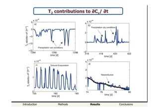
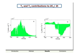
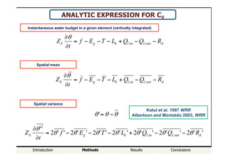
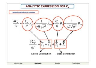
Contributions to ∂Cv/ ∂t
500 1000 1500
0
0.2
0.4
0.6
0.8
1
time [day]
[-]
T1
abiotic-var
500 1000 1500
0
0.2
0.4
0.6
0.8
1
time [day]
[-]
T2
abiotic-µ
500 1000 1500
0
0.2
0.4
0.6
0.8
1
time [day]
[-]
T3
biotic-µ
500 1000 1500
0
0.2
0.4
0.6
0.8
1
time [day]
[-]
T4
biotic-var
T2 – Abiotic Variance T1 – Abiotic Mean
T3 – Biotic Mean T4 – Biotic Variance
[-]
[-][-]
[-]

22. Introduction Methods Results Conclusions
T1 contributions to ∂Cv/ ∂t

23. Introduction Methods Results Conclusions
T2 contributions to ∂Cv/ ∂t

24. Introduction Methods Results Conclusions
T3 and T4 contributions to ∂Cv/ ∂t

25. Introduction Methods Results Conclusions
RESULTS
UMBS
Θ
Cv(Θ)
Frequency
Frequency
Θ
Fully Biotic
Fully Abiotic

26. Results
Cv(Θ)
Θ
Cv(Θ)Cv(Θ)
UMBS (MI)
DAVOS (CH)
RIETHOLZBACH (CH) SAN ROSSORE (IT)
VAIRA RANCH (CA)
LUCKY HILLS (AZ)
Θ
Cv(Θ)Cv(Θ)Cv(Θ)
HOMOGENOUS SOIL

27. Results
Cv(Θ)
Θ
Cv(Θ)Cv(Θ)
UMBS (MI)
DAVOS (CH)
RIETHOLZBACH (CH)
SAN ROSSORE (IT)
VAIRA RANCH (CA)
LUCKY HILLS (AZ)
Θ
Cv(Θ)Cv(Θ)
Cv(Θ)
HETEROG. LOAM

28. Results
Cv(Θ)
Θ
Cv(Θ)
Cv(Θ)
UMBS (MI)
DAVOS (CH)
RIETHOLZBACH (CH) SAN ROSSORE (IT)
VAIRA RANCH (CA)
LUCKY HILLS (AZ)
Θ
Cv(Θ)Cv(Θ)
Cv(Θ)
FULLY HETEROG.

29. Introduction Methods Results Conclusions
ABIOTIC VS. BIOTIC CONTROLS
43
21
TTB
TTA
+=
+=
WETNESS INDEX WETNESS INDEX

30. SUMMARY
! Abio%c' (A)' controls' are' always' larger' than' bio%c' (B)' ones' and' are'
dominant' in' wet' climates' The' maximum' of' B/A' is' obtained' for'
Mediterranean'climates.'
! The' rela%on' between' Cv' and Θ was' found' to' be' unique' and' well'
described' by' an' exponen%al' or' linear' func%on' for' the' Swiss' loca%ons'
regardless'of'soil'proper%es.''
! Strong'hystere%c'cycles'were'observed'for'the'Mediterranean'loca%ons'
and,'to'a'lesser'extent,'at'the'UMBS'for'homogenous'soil'textural'proper%es.''
! Heterogeneity' in' soil' proper%es' increases' Cv' to' magnitudes'
commensurable'with'field'observa%ons'and'tends'to'mask'hysteresis'in'all'of'
the'loca%ons.'
! Heterogeneity'in'soil'can'obscure'or'hide'clima%c'and'bio%c'controls'of'
soil'moisture'spa%oItemporal'variability.''

31. Thanks for your
attention !
Fatichi et al., 2015, WRR