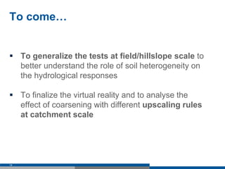
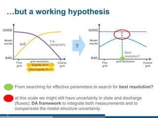
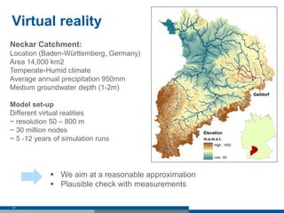
This document provides an overview of a project studying the effects of subsurface heterogeneity at hillslope scales using the Parflow modeling system. It discusses motivations to better understand upscaling rules when applying distributed hydrological models with heterogeneous parameters. Initial tests are presented examining the impact of soil property variability on soil moisture and discharge dynamics for flat fields and hillslopes. Preliminary results show that state dynamics are well represented by homogeneous models, but heterogeneity increases non-equilibrium and impacts could depend on the ergodic or non-ergodic nature of the domain. Further work is planned to generalize the tests and analyze coarsening effects at the catchment scale.

1. 24/09/2015
Padova (IT)
On the role of subsurface
heterogeneity at hillslope
scale with Parflow
Gabriele Baroni
Sabine Attinger

2. Outline
 Quick overview of the project
 Motivations in our research unit
 The effect of soil heterogeneity at field/hillslope
 Outlook
2

3. Overview project
German funded project (DFG)
"Data Assimilation for Improved Characterization of
Fluxes across Compartmental Interfaces“
Seven research units working on different compartments
of the terrestrial system
3
http://www.for2131.de/home-en

4. Overview project and our unit
1. To create a virtual reality at catchment
scale with an integrated model (TerrSysMP)
2. Coarsening the model with different
upscaling rules and see the effects
3. To develop a unified data assimilation
framework to improve the performance of
the model
• which measurements to integrate?
• how?
4
Test at
small
scales

5. Motivations
heterogeneity and scaling effects
 Whenever we apply the current distributed
models (e.g. Richards eq.) we assume uniform
parameters within the grid
 Whatever is the scale of application (lab, field,
catchment) we do an upscaling exercise
5

6. Research questions
in this upscaling exercise?
 we have to find upscaling rules/effective
parameters
• different results functions of domain set-up,
parameters distributions, boundary conditions etc.
• Holy Grail of hydrology…worth searching for
even if a general solution might ultimate prove
impossible to find (Beven, 2006)
6

7. Hillslope
Rain/runoff
Flat field
Infiltration/drainage
Tests at field/hillslope with Parflow
Variability in soil properties (~Fiori and Russo, 2007)
7
1 Homogeneous
2
s2= 0.3
~ergodic domain = 33 * Integral scale
3 ~non-ergodic domain = 5 * Integral scale
4
s2= 1.0
~ergodic domain = 33 * Integral scale
5 ~non-ergodic domain = 5 * Integral scale

8. Same mean but variability
Flat field
Infiltration/drainage at 10 cm depths
8
Homogeneous
Mean and variance of soil moisture
and pressure over the plan
- 10 cm - 10 cm

9. Flat field:
mean soil moisture and pressure
9
• Soil moisture dynamics well
represented by the homogeneous
counterpart
• To check if differences are within
statistics of the random fields
(single realization vs. ensemble of
50 realizations)

10. Flat field:
mean soil moisture and pressure
10
• Differences if s2 increases
• To check effect of this dynamic
non-equilibrium in longer term
t0
t1
t2
t0
t1
t2

11. Hillslope
storage-discharge
11
• Storage dynamics well
represented by the homogeneous
counterpart
• To check if differences are within
statistics of the random fields
(single realization vs. ensemble
of 50 realizations)

12. Hillslope
storage-discharge
12
• Storage dynamics well
represented by the homogeneous
counterpart
• To check if differences are within
statistics of the random fields
(single realization vs. ensemble
of 50 realizations)
• Heterogeneity = faster responses
• Some differences especially if
non-ergodic

13. To summarize so far…
With an homogeneous counterpart
 state dynamic well represented (i.e., soil
moisture or water storage)
 variability increases dynamic non–equilibrium
but to test implications at longer term
 non-ergodicity - more than variability - precludes
the use of general upscaling rules
13

14. To come…
 To generalize the tests at field/hillslope scale to
better understand the role of soil heterogeneity on
the hydrological responses
 To finalize the virtual reality and to analyse the
effect of coarsening with different upscaling rules
at catchment scale
14

15. …but a working hypothesis
15
Model
results
GOOD
BAD
Fine
grid
Coarse
grid
e.g.,
topographysoil
Ergodic D>>I
grid resolution
 From searching for effective parameters to search for best resolution?
grid resolution
GOOD
BAD
Fine
grid
Coarse
grid
Model
results
?
Best
resolution?
Non-ergodic D ~ I
 at this scale we might still have uncertainty in state and discharge
(fluxes): DA framework to integrate both measurements and to
compensate the model structure uncertainty

16. Thank you for the attention
16

17. Virtual reality
17
Neckar Catchment:
Location (Baden-Württemberg, Germany)
Area 14,000 km2
Temperate-Humid climate
Average annual precipitation 950mm
Medium groundwater depth (1-2m)
Model set-up
Different virtual realities
~ resolution 50 – 800 m
~ 30 million nodes
~ 5 -12 years of simulation runs
 We aim at a reasonable approximation
 Plausible check with measurements

18. Details of model set-up
18
1 Homogeneous
2
s2= 0.3
~ergodic domain = 33 * Integral scale
3 ~non-ergodic domain = 5 * Integral scale
4
s2= 1.0
~ergodic domain = 33 * Integral scale
5 ~non-ergodic domain = 5 * Integral scale
Soil
Domain
50 x 50 x 50 nodes
1 m resolutions xy
dZ verticalbedrock
1.4 m
18.6 m
50 m
50 m

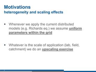
19. Details about soil variability (~Fiori and Russo, 2007)
19
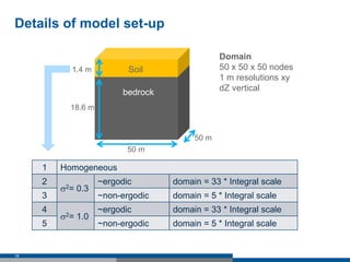
Homogeneous
s2 = 0.3 s2 = 1.0
s2 CV s2 CV
Ksat [m/h] 0.02 (geom.) 0.3 0.6 1.0 1.3
a [m-1] 3.5 (geom.) 0.2 0.4 0.5 0.8
n [-] 2.0 (arithmetic) 0.02 0.05 0.05 0.1
qs [-] 0.42 (arithmetic) 0.001 0.05 0.002 0.1
Ksat [m/h] a [m-1] n [-] qs [-]
Ksat [m/h] 1
a [m-1] 0.8 1
n [-] 0.4 0.5 1
qs [-] -0.4 -0.2 -0.6 1
Correlation matrix

20. Energy and mass fluxes in TerrSysMP
20
Gasper al, 2015