Download to read offline

![Carlo Gregoretti25/5/2017 Mekelle University - Debris Flows
The linear concentration depends on c. The quantities Y and D are the
two parameters of TRENT2D and rule the flow resistance of the mixture.
They vary in the following range:
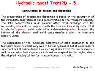
The bottom shear stress is obtained through the rheological law proposed
by Bagnold (1954) for the grain-inertial regime.
15 Y 25 e 30 D 40°
Closure equation for the bottom shear stress
Hydraulic model Trent2D - 3
= 1/[(cb/ c) 1/3 – 1];
Y = h/(d a 1/3);
D = dynamic friction angle;
a = constant of the collisional shear stress
expression provided by Bagnold (1954).](https://image.slidesharecdn.com/08modelliidraulicicolataen-170526125202/85/08-modelli-idraulici_colata_en-5-320.jpg)
![Carlo Gregoretti25/5/2017 Mekelle University - Debris Flows
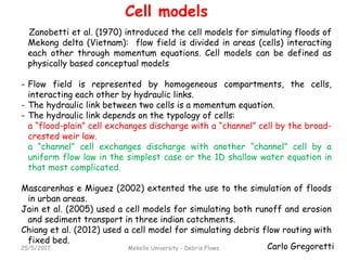
The solid concentration is computed by means of a transport capacity
equation:
Closure equation for the solid concentration
= transport dimensionless parameter
The parameter is computed by the code according to the following
equation depending on the two parameters, Y and D, theoretically valid
only in uniform flow conditions:
transport capacity:
solid concentration or discharge
in uniform flow conditions
Hydraulic model Trent2D - 4
= 1/[(cb/ c) 1/3 – 1]; Y = h/(d a 1/3); D = dynamic friction angle; ib = bed slope; cb =
dry bed solid concentration at rest; a = constant of the collisional shear stress
expression provided by Bagnold (1954); = (s - w)/w.](https://image.slidesharecdn.com/08modelliidraulicicolataen-170526125202/85/08-modelli-idraulici_colata_en-6-320.jpg)

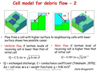
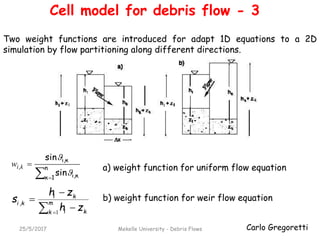
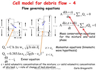
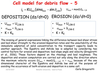
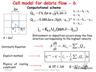

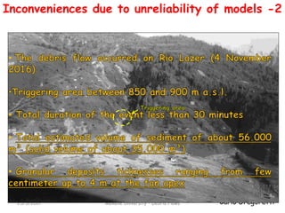
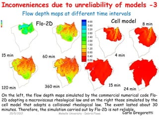
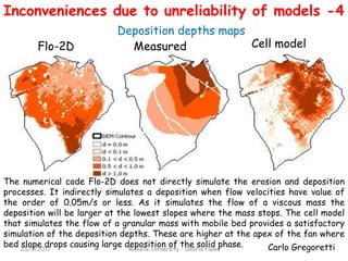


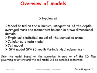
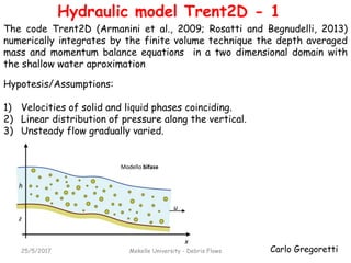
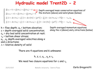
The document discusses different models for simulating debris flows, focusing on two models: the Trent2D hydraulic model and a cell model. The Trent2D model numerically integrates the depth-averaged mass and momentum balance equations using closure equations for solid concentration and bottom shear stress. The cell model represents the flow field as interacting cells linked by uniform flow or weir flow equations, and simulates erosion and deposition based on velocity and slope thresholds. Both models make simplifying assumptions that could lead to incorrect results if not physically suitable for the problem being modeled.


