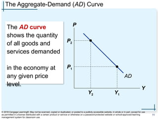
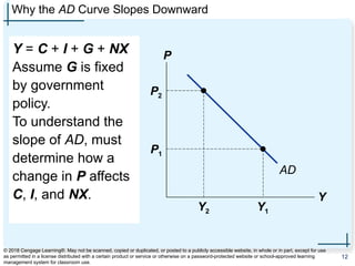
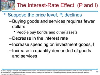
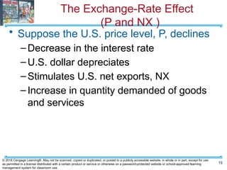
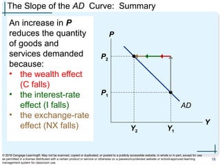
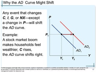
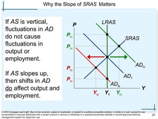
Premium PowerPoint Slides by:
V. Andreea CHIRITESCU
Eastern Illinois University
N. GREGORY MANKIW
PRINCIPLES OF
ECONOMICS
Eight Edition
Aggregate Demand
and Aggregate Supply
CHAPTER
33
© 2018 Cengage Learning®. May not be scanned, copied or duplicated, or posted to a publicly accessible website, in whole or in part, except for use
as permitted in a license distributed with a certain product or service or otherwise on a password-protected website or school-approved learning
management system for classroom use.
1
Introduction
• This chapter has introduced the model of
aggregate demand and aggregate supply
– Helps explain economic fluctuations.
• Keep in mind:
– These fluctuations are deviations from the long-
run trends explained by the models we learned
in previous chapters.
• In the next chapter
– How policymakers can affect aggregate demand
with fiscal and monetary policy.
2
© 2018 Cengage Learning®. May not be scanned, copied or duplicated, or posted to a publicly accessible website, in whole or in part, except for use
as permitted in a license distributed with a certain product or service or otherwise on a password-protected website or school-approved learning
management system for classroom use.
Look for the answers to these questions:
• What are economic fluctuations? What are
their characteristics?
• How does the model of aggregate demand and
aggregate supply explain economic
fluctuations?
• Why does the Aggregate-Demand curve slope
downward? What shifts the AD curve?
• What is the slope of the Aggregate-Supply
curve in the short run? In the long run?
What shifts the AS curve(s)?
3
© 2018 Cengage Learning®. May not be scanned, copied or duplicated, or posted to a publicly accessible website, in whole or in part, except for use
as permitted in a license distributed with a certain product or service or otherwise on a password-protected website or school-approved learning
management system for classroom use.
Introduction
• Real GDP over the long run
–Grows about 3% per year on average
• GDP in the short run
–Fluctuates around its trend
• Recessions
–Periods of falling real incomes and rising
unemployment
• Depressions
–Severe recessions (very rare)
4
© 2018 Cengage Learning®. May not be scanned, copied or duplicated, or posted to a publicly accessible website, in whole or in part, except for use
as permitted in a license distributed with a certain product or service or otherwise on a password-protected website or school-approved learning
management system for classroom use.
Three Facts About Economic Fluctuations
FACT 1: Economic fluctuations are irregular and unpredictable
5
© 2018 Cengage Learning®. May not be scanned, copied or duplicated, or posted to a publicly accessible website, in whole or in part, except for use
as permitted in a license distributed with a certain product or service or otherwise on a password-protected website or school-approved learning
management system for classroom use.
Three Facts About Economic Fluctuations
FACT 2: Most macroeconomic quantities fluctuate together.
6
© 2018 Cengage Learning®. May not be scanned, copied or duplicated, or posted to a publicly accessible website, in whole or in part, except for use
as permitted in a license distributed with a certain product or service or otherwise on a password-protected website or school-approved learning
management system for classroom use.
Three Facts About Economic Fluctuations
FACT 3: As output falls, unemployment rises.
7
© 2018 Cengage Learning®. May not be scanned, copied or duplicated, or posted to a publicly accessible website, in whole or in part, except for use
as permitted in a license distributed with a certain product or service or otherwise on a password-protected website or school-approved learning
management system for classroom use.
Classical Economics—A Recap
• Classical economics:
–The Classical Dichotomy, the separation
of variables into two groups:
• Real – quantities, relative prices
• Nominal – measured in terms of money
–The neutrality of money: Changes in the
money supply affect nominal but not real
variables
8
© 2018 Cengage Learning®. May not be scanned, copied or duplicated, or posted to a publicly accessible website, in whole or in part, except for use
as permitted in a license distributed with a certain product or service or otherwise on a password-protected website or school-approved learning
management system for classroom use.
Classical Economics—A Recap
• Classical theory
–Describes the world in the long run, but
not the short run
• In the short run
–Changes in nominal variables (like the
money supply or P ) can affect real
variables (like Y or the u-rate).
–We use a new model…
9
© 2018 Cengage Learning®. May not be scanned, copied or duplicated, or posted to a publicly accessible website, in whole or in part, except for use
as permitted in a license distributed with a certain product or service or otherwise on a password-protected website or school-approved learning
management system for classroom use.
Model of Aggregate Demand and Aggregate Supply
P
Y
AD
SRAS
P1
Y1
The price
level
Real GDP, the
quantity of output
“Aggregate
Demand”
“Short-Run
Aggregate Supply”
The model
determines the
equilibrium
price level
and equilibrium
output (real GDP).
© 2018 Cengage Learning®. May not be scanned, copied or duplicated, or posted to a publicly accessible website, in whole or in part, except for use
as permitted in a license distributed with a certain product or service or otherwise on a password-protected website or school-approved learning
management system for classroom use.
10
The Aggregate-Demand (AD) Curve
The AD curve
shows the quantity
of all goods and
services demanded
in the economy at
any given price
level.
P
Y
AD
P1
Y1
P2
Y2
© 2018 Cengage Learning®. May not be scanned, copied or duplicated, or posted to a publicly accessible website, in whole or in part, except for use
as permitted in a license distributed with a certain product or service or otherwise on a password-protected website or school-approved learning
management system for classroom use.
11
Why the AD Curve Slopes Downward
Y = C + I + G + NX
Assume G is fixed
by government
policy.
To understand the
slope of AD, must
determine how a
change in P affects
C, I, and NX.
P
Y
AD
P1
Y1
P2
Y2 Y1
© 2018 Cengage Learning®. May not be scanned, copied or duplicated, or posted to a publicly accessible website, in whole or in part, except for use
as permitted in a license distributed with a certain product or service or otherwise on a password-protected website or school-approved learning
management system for classroom use.
12
The Wealth Effect (P and C )
• Suppose the price level, P, declines
–Increase in the real value of money
–Consumers are wealthier
–Increase in consumer spending, C
–Increase in quantity demanded of goods
and services
13
© 2018 Cengage Learning®. May not be scanned, copied or duplicated, or posted to a publicly accessible website, in whole or in part, except for use
as permitted in a license distributed with a certain product or service or otherwise on a password-protected website or school-approved learning
management system for classroom use.
The Interest-Rate Effect (P and I)
• Suppose the price level, P, declines
–Buying goods and services requires fewer
dollars
• People buy bonds and other assets
–Decrease in the interest rate
–Increase spending on investment goods, I
–Increase in quantity demanded of goods
and services
14
© 2018 Cengage Learning®. May not be scanned, copied or duplicated, or posted to a publicly accessible website, in whole or in part, except for use
as permitted in a license distributed with a certain product or service or otherwise on a password-protected website or school-approved learning
management system for classroom use.
The Exchange-Rate Effect
(P and NX )
• Suppose the U.S. price level, P, declines
–Decrease in the interest rate
–U.S. dollar depreciates
–Stimulates U.S. net exports, NX
–Increase in quantity demanded of goods
and services
15
© 2018 Cengage Learning®. May not be scanned, copied or duplicated, or posted to a publicly accessible website, in whole or in part, except for use
as permitted in a license distributed with a certain product or service or otherwise on a password-protected website or school-approved learning
management system for classroom use.
The Slope of the AD Curve: Summary
An increase in P
reduces the quantity
of goods and
services demanded
because:
• the wealth effect
(C falls)
• the interest-rate
effect (I falls)
• the exchange-rate
effect (NX falls)
P
Y
AD
P1
Y1
P2
Y2
© 2018 Cengage Learning®. May not be scanned, copied or duplicated, or posted to a publicly accessible website, in whole or in part, except for use
as permitted in a license distributed with a certain product or service or otherwise on a password-protected website or school-approved learning
management system for classroom use.
16
Why the AD Curve Might Shift
Any event that changes
C, I, G, or NX—except
a change in P—will shift
the AD curve.
Example:
A stock market boom
makes households feel
wealthier, C rises,
the AD curve shifts right.
P
Y
AD1
AD2
Y2
P1
Y1
© 2018 Cengage Learning®. May not be scanned, copied or duplicated, or posted to a publicly accessible website, in whole or in part, except for use
as permitted in a license distributed with a certain product or service or otherwise on a password-protected website or school-approved learning
management system for classroom use.
17
Why the AD Curve Might Shift
• Changes in C
– Stock market boom/crash
– Preferences re: consumption/saving tradeoff
– Tax hikes/cuts
18
© 2018 Cengage Learning®. May not be scanned, copied or duplicated, or posted to a publicly accessible website, in whole or in part, except for use
as permitted in a license distributed with a certain product or service or otherwise on a password-protected website or school-approved learning
management system for classroom use.
• Changes in I
– Firms buy new computers, equipment, factories
– Expectations, optimism/pessimism
– Interest rates,
– Monetary policy,
– Investment Tax Credit or other tax incentives
Why the AD Curve Might Shift
• Changes in G
– Federal spending, e.g., defense
– State & local spending, e.g., roads, schools
19
© 2018 Cengage Learning®. May not be scanned, copied or duplicated, or posted to a publicly accessible website, in whole or in part, except for use
as permitted in a license distributed with a certain product or service or otherwise on a password-protected website or school-approved learning
management system for classroom use.
• Changes in NX
– Booms/recessions in countries that buy our
exports
– Appreciation/depreciation resulting from
international speculation in foreign exchange
market
Active Learning 1 Answers
A. A ten-year-old investment tax credit expires.
– I falls, AD curve shifts left.
B. The U.S. exchange rate falls.
– NX rises, AD curve shifts right.
C. A fall in prices increases the real value of
consumers’ wealth.
– Move down along AD curve (wealth-effect).
D. State governments replace their sales taxes with
new taxes on interest, dividends, and capital
gains.
– C rises, AD shifts right.
20
© 2018 Cengage Learning®. May not be scanned, copied or duplicated, or posted to a publicly accessible website, in whole or in part, except for use
as permitted in a license distributed with a certain product or service or otherwise on a password-protected website or school-approved learning
management system for classroom use.
The Aggregate-Supply (AS ) Curves
The AS curve shows
the total quantity of
goods and services
firms produce and
sell at any given
price level.
AS is:
 upward-sloping in
short run
 vertical in long run
P
Y
SRAS
LRAS
© 2018 Cengage Learning®. May not be scanned, copied or duplicated, or posted to a publicly accessible website, in whole or in part, except for use
as permitted in a license distributed with a certain product or service or otherwise on a password-protected website or school-approved learning
management system for classroom use.
21
The Long-Run Aggregate-Supply Curve (LRAS)
The natural rate of
output (YN) is the amount
of output the economy
produces when
unemployment is at its
natural rate.
Also called
potential output
or
full-employment output.
P
Y
LRAS
YN
© 2018 Cengage Learning®. May not be scanned, copied or duplicated, or posted to a publicly accessible website, in whole or in part, except for use
as permitted in a license distributed with a certain product or service or otherwise on a password-protected website or school-approved learning
management system for classroom use.
22
Why LRAS Is Vertical
YN determined by the
economy’s stocks of
labor, capital, and natural
resources, and on the
level of technology.
An increase in P
does not affect any of
these, so it does not
affect YN.
(Classical dichotomy)
P
Y
LRAS
P1
P2
YN
© 2018 Cengage Learning®. May not be scanned, copied or duplicated, or posted to a publicly accessible website, in whole or in part, except for use
as permitted in a license distributed with a certain product or service or otherwise on a password-protected website or school-approved learning
management system for classroom use.
23
Why the LRAS Curve Might Shift
Any event that
changes any of the
determinants of YN
will shift LRAS.
Example:
Immigration
increases L,
causing YN to rise.
P
Y
LRAS1
YN
LRAS2
YN
’
© 2018 Cengage Learning®. May not be scanned, copied or duplicated, or posted to a publicly accessible website, in whole or in part, except for use
as permitted in a license distributed with a certain product or service or otherwise on a password-protected website or school-approved learning
management system for classroom use.
24
Why the LRAS Curve Might Shift
• Changes in L or natural rate of
unemployment
–Immigration
–Baby-boomers retire
–Government policies reduce natural u-rate
25
© 2018 Cengage Learning®. May not be scanned, copied or duplicated, or posted to a publicly accessible website, in whole or in part, except for use
as permitted in a license distributed with a certain product or service or otherwise on a password-protected website or school-approved learning
management system for classroom use.
• Changes in K or H
–Investment in factories, equipment
–More people get college degrees
–Factories destroyed by a hurricane
Why the LRAS Curve Might Shift
• Changes in natural resources
–Discovery of new mineral deposits
–Reduction in supply of imported oil
–Changing weather patterns that affect
agricultural production
26
© 2018 Cengage Learning®. May not be scanned, copied or duplicated, or posted to a publicly accessible website, in whole or in part, except for use
as permitted in a license distributed with a certain product or service or otherwise on a password-protected website or school-approved learning
management system for classroom use.
• Changes in technology
–Productivity improvements from
technological progress
LRAS1990
Using AD & AS to Depict Long-Run Growth & Inflation
Over the long run,
tech. progress
shifts LRAS to the
right
and growth in the
money supply
shifts AD to the
right.
Result:
ongoing inflation
and growth in
output.
P
Y
AD2000
LRAS2000
AD1990
Y2000
Y1990
AD2010
LRAS2010
Y2010
P1990
P2000
P2010
© 2018 Cengage Learning®. May not be scanned, copied or duplicated, or posted to a publicly accessible website, in whole or in part, except for use
as permitted in a license distributed with a certain product or service or otherwise on a password-protected website or school-approved learning
management system for classroom use.
27
Short Run Aggregate Supply (SRAS)
The SRAS curve
is upward sloping:
Over the period
of 1–2 years,
an increase in P
causes an increase
in the quantity of
goods and services
supplied.
P
Y
SRAS
Y2
P1
Y1
P2
© 2018 Cengage Learning®. May not be scanned, copied or duplicated, or posted to a publicly accessible website, in whole or in part, except for use
as permitted in a license distributed with a certain product or service or otherwise on a password-protected website or school-approved learning
management system for classroom use.
28
Why the Slope of SRAS Matters
If AS is vertical,
fluctuations in AD
do not cause
fluctuations in
output or
employment.
If AS slopes up,
then shifts in AD
do affect output and
employment.
P
Y
AD1
SRAS
LRAS
ADhi
ADlo
Y1
Plo
Ylo
Phi
Yhi
Phi
Plo
© 2018 Cengage Learning®. May not be scanned, copied or duplicated, or posted to a publicly accessible website, in whole or in part, except for use
as permitted in a license distributed with a certain product or service or otherwise on a password-protected website or school-approved learning
management system for classroom use.
29
Three Theories of SRAS
• Theories that explain why the AS curve
slopes upward in short-run:
–Sticky-wage theory
–Sticky-price theory
–Misperceptions theory
• In each, some type of market imperfection:
Output deviates from its natural rate when
the actual price level deviates from the price
level people expected.
30
© 2018 Cengage Learning®. May not be scanned, copied or duplicated, or posted to a publicly accessible website, in whole or in part, except for use
as permitted in a license distributed with a certain product or service or otherwise on a password-protected website or school-approved learning
management system for classroom use.
1. The Sticky-Wage Theory
• Imperfection:
–Nominal wages are sticky in the short run,
they adjust sluggishly.
• Due to labor contracts, social norms
• Firms and workers set the nominal wage in
advance based on PE, the price level they
expect to prevail.
31
© 2018 Cengage Learning®. May not be scanned, copied or duplicated, or posted to a publicly accessible website, in whole or in part, except for use
as permitted in a license distributed with a certain product or service or otherwise on a password-protected website or school-approved learning
management system for classroom use.
1. The Sticky-Wage Theory
• If P > PE,
–Revenue is higher, but labor cost is not.
–Production is more profitable, so firms
increase output and employment.
Hence, higher P causes higher Y, so the SRAS
curve slopes upward.
32
© 2018 Cengage Learning®. May not be scanned, copied or duplicated, or posted to a publicly accessible website, in whole or in part, except for use
as permitted in a license distributed with a certain product or service or otherwise on a password-protected website or school-approved learning
management system for classroom use.
2. The Sticky-Price Theory
• Imperfection:
–Many prices are sticky in the short run.
• Due to menu costs, the costs of adjusting
prices.
• Examples: cost of printing new menus,
the time required to change price tags
–Firms set sticky prices in advance based
on PE
33
© 2018 Cengage Learning®. May not be scanned, copied or duplicated, or posted to a publicly accessible website, in whole or in part, except for use
as permitted in a license distributed with a certain product or service or otherwise on a password-protected website or school-approved learning
management system for classroom use.
2. The Sticky-Price Theory
• Suppose the Fed increases the money supply
unexpectedly
– In the long run, P will rise
– In the short run:
• Firms without menu costs can raise their prices
immediately
• Firms with menu costs wait to raise prices. With
relatively low prices: increase demand for their
products: increase output and employment
Hence, higher P is associated with higher Y, so the
SRAS curve slopes upward.
34
© 2018 Cengage Learning®. May not be scanned, copied or duplicated, or posted to a publicly accessible website, in whole or in part, except for use
as permitted in a license distributed with a certain product or service or otherwise on a password-protected website or school-approved learning
management system for classroom use.
3. The Misperceptions Theory
• Imperfection:
– Firms may confuse changes in P with changes in
the relative price of the products they sell.
• If P rises above PE
– A firm sees its price rise before realizing all
prices are rising.
• The firm may believe its relative price is rising,
and may increase output and employment.
So, an increase in P can cause an increase in Y, making
the SRAS curve upward-sloping.
35
© 2018 Cengage Learning®. May not be scanned, copied or duplicated, or posted to a publicly accessible website, in whole or in part, except for use
as permitted in a license distributed with a certain product or service or otherwise on a password-protected website or school-approved learning
management system for classroom use.
What the 3 Theories Have in Common:
• In all 3 theories, Y deviates from YN when
P deviates from PE.
36
© 2018 Cengage Learning®. May not be scanned, copied or duplicated, or posted to a publicly accessible website, in whole or in part, except for use
as permitted in a license distributed with a certain product or service or otherwise on a password-protected website or school-approved learning
management system for classroom use.
Y = YN + a(P – PE)
Output
Natural rate
of output
(long-run)
a > 0,
measures
how much Y
responds to
unexpected
changes in P
Actual
price level
Expected
price level
What the 3 Theories Have in Common:
P
Y
SRAS
YN
When P > PE
Y > YN
When P < PE
Y < YN
PE
the expected
price level
Y = YN + a(P – PE)
© 2018 Cengage Learning®. May not be scanned, copied or duplicated, or posted to a publicly accessible website, in whole or in part, except for use
as permitted in a license distributed with a certain product or service or otherwise on a password-protected website or school-approved learning
management system for classroom use.
37
SRAS and LRAS
• The imperfections in these theories are
temporary. Over time,
–Sticky wages and prices become flexible
–Misperceptions are corrected
• In the LR,
–PE = P
–AS curve is vertical
38
© 2018 Cengage Learning®. May not be scanned, copied or duplicated, or posted to a publicly accessible website, in whole or in part, except for use
as permitted in a license distributed with a certain product or service or otherwise on a password-protected website or school-approved learning
management system for classroom use.
LRAS
SRAS and LRAS
In the long run,
PE = P
and
Y = YN.
P
Y
SRAS
PE
YN
Y = YN + a(P – PE)
© 2018 Cengage Learning®. May not be scanned, copied or duplicated, or posted to a publicly accessible website, in whole or in part, except for use
as permitted in a license distributed with a certain product or service or otherwise on a password-protected website or school-approved learning
management system for classroom use.
39
Why the SRAS Curve Might Shift
Everything that shifts
LRAS shifts SRAS,
too.
Also, PE shifts SRAS:
If PE rises,
workers & firms set
higher wages.
At each P,
production is less
profitable, Y falls,
SRAS shifts left.
LRAS
P
Y
SRAS
PE
YN
SRAS
PE
© 2018 Cengage Learning®. May not be scanned, copied or duplicated, or posted to a publicly accessible website, in whole or in part, except for use
as permitted in a license distributed with a certain product or service or otherwise on a password-protected website or school-approved learning
management system for classroom use.
40
The Long-Run Equilibrium
In the long-run
equilibrium,
PE = P,
Y = YN ,
and unemployment
is at its natural rate.
P
Y
AD
SRAS
PE
LRAS
YN
© 2018 Cengage Learning®. May not be scanned, copied or duplicated, or posted to a publicly accessible website, in whole or in part, except for use
as permitted in a license distributed with a certain product or service or otherwise on a password-protected website or school-approved learning
management system for classroom use.
41
Economic Fluctuations
• Four steps to analyzing economic
fluctuations:
1. Determine whether the event shifts AD or
AS.
2. Determine whether curve shifts left or right.
3. Use AD–AS diagram to see how the shift
changes Y and P in the short run.
4. Use AD–AS diagram to see how economy
moves from new SR equilibrium to new LR
equilibrium .
42
© 2018 Cengage Learning®. May not be scanned, copied or duplicated, or posted to a publicly accessible website, in whole or in part, except for use
as permitted in a license distributed with a certain product or service or otherwise on a password-protected website or school-approved learning
management system for classroom use.
LRAS
YN
The Effects of a Shift in AD
Event: Stock market crash
1. Affects C, AD curve
2. C falls, so AD shifts left
3. SR equilibrium at B.
P and Y lower,
unemployment higher
4. Over time, PE falls,
SRAS shifts right,
until LR equilibrium at
C. Y and
unemployment back
at initial levels.
P
Y
AD1
SRAS1
AD2
SRAS2
P1 A
P2
Y2
B
P3 C
© 2018 Cengage Learning®. May not be scanned, copied or duplicated, or posted to a publicly accessible website, in whole or in part, except for use
as permitted in a license distributed with a certain product or service or otherwise on a password-protected website or school-approved learning
management system for classroom use.
43
Two Big AD Shifts: 1.The Great Depression
• From 1929–1933,
money supply fell 28%
due to problems in
banking system
• stock prices fell 90%,
reducing C and I
• Y fell 27%
• P fell 22%
• Unemployment rate
rose from 3% to 25%
44
© 2018 Cengage Learning®. May not be scanned, copied or duplicated, or posted to a publicly accessible website, in whole or in part, except for use
as permitted in a license distributed with a certain product or service or otherwise on a password-protected website or school-approved learning
management system for classroom use.
1929
1930
1931
1932
1933
1934
550
600
650
700
750
800
850
900
U.S. Real GDP,
billions of 2000 dollars
Two Big AD Shifts: 2.The World War II Boom
• From 1939–1944,
• government outlays
rose from $9.1 billion
to $91.3 billion
• Y rose 90%
• P rose 20%
• unemployment fell
from 17% to 1%
45
© 2018 Cengage Learning®. May not be scanned, copied or duplicated, or posted to a publicly accessible website, in whole or in part, except for use
as permitted in a license distributed with a certain product or service or otherwise on a password-protected website or school-approved learning
management system for classroom use.
1939
1940
1941
1942
1943
1944
800
1,000
1,200
1,400
1,600
1,800
2,000
U.S. Real GDP,
billions of 2000 dollars
Active Learning 2 Working with the model
Draw the AD-SRAS-LRAS diagram for the
U.S. economy starting in a long-run
equilibrium.
• A boom occurs in Canada. Use your
diagram to determine the SR and LR effects
on U.S. GDP, the price level, and
unemployment.
46
© 2018 Cengage Learning®. May not be scanned, copied or duplicated, or posted to a publicly accessible website, in whole or in part, except for use
as permitted in a license distributed with a certain product or service or otherwise on a password-protected website or school-approved learning
management system for classroom use.
Active Learning 2 Answers
47
© 2018 Cengage Learning®. May not be scanned, copied or duplicated, or posted to a publicly accessible website, in whole or in part, except for use
as permitted in a license distributed with a certain product or service or otherwise on a password-protected website or school-approved learning
management system for classroom use.
Event: Boom in Canada
1. Affects NX, AD curve
2. Shifts AD right
3. SR equilibrium at point
B. P and Y higher,
unemployment lower
4. Over time, PE rises,
SRAS shifts left, until
LR equilibrium at C.
Y and unemployment
back at initial levels.
LRAS
YN
P
Y
AD2
SRAS2
AD1
SRAS1
P1
P3 C
P2
Y2
B
A
The Great Recession of 2008–2009
• Large contractionary shift in AD
–Real GDP fell sharply
• By 4.2% between the forth quarter of 2007
and the second quarter of 2009
–Employment fell sharply
• Unemployment rate rose from 4.4% in May
2007 to 10.0% in October 2009
• The housing market played a central role
in this recession…
48
© 2018 Cengage Learning®. May not be scanned, copied or duplicated, or posted to a publicly accessible website, in whole or in part, except for use
as permitted in a license distributed with a certain product or service or otherwise on a password-protected website or school-approved learning
management system for classroom use.
CASE STUDY: The Great Recession of 2008–2009
49
© 2018 Cengage Learning®. May not be scanned, copied or duplicated, or posted to a publicly accessible website, in whole or in part, except for use
as permitted in a license distributed with a certain product or service or otherwise on a password-protected website or school-approved learning
management system for classroom use.
2000 2001 2002 2003 2004 2005 2006 2007 2008 2009 2010 2011
80
100
120
140
160
180
200
220 Case-Shiller Home Price Index
2000
=
100
The Great Recession of 2008–2009
• Rising house prices during 2002–2006
due to:
–Low interest rates
–Easier credit for “sub-prime” borrowers
–Government policies to increase
homeownership
–Securitization of mortgages
50
© 2018 Cengage Learning®. May not be scanned, copied or duplicated, or posted to a publicly accessible website, in whole or in part, except for use
as permitted in a license distributed with a certain product or service or otherwise on a password-protected website or school-approved learning
management system for classroom use.
The Great Recession of 2008–2009
• Securitization of mortgages:
–Investment banks purchased mortgages
from lenders,
• Created securities backed by these
mortgages,
• Sold the securities to banks, insurance
companies, and other investors.
–Mortgage-backed securities perceived as
safe, since house prices “never fall”
51
© 2018 Cengage Learning®. May not be scanned, copied or duplicated, or posted to a publicly accessible website, in whole or in part, except for use
as permitted in a license distributed with a certain product or service or otherwise on a password-protected website or school-approved learning
management system for classroom use.
The Great Recession of 2008–2009
• Consequences of 2006–2009 housing
market crash:
– Millions of homeowners “underwater”—
owed more than house was worth.
– Millions of mortgage defaults and
foreclosures.
– Banks selling foreclosed houses increased
surplus and downward price pressures.
– Housing crash badly damaged construction
industry: 2010 unemployment rate was
20.6% in construction vs. 9.6% overall.
52
© 2018 Cengage Learning®. May not be scanned, copied or duplicated, or posted to a publicly accessible website, in whole or in part, except for use
as permitted in a license distributed with a certain product or service or otherwise on a password-protected website or school-approved learning
management system for classroom use.
The Great Recession of 2008–2009
• Consequences of 2006–2009 housing
market crash:
– Mortgage-backed securities became “toxic,”
• Heavy losses for institutions that purchased
them,
• Widespread failures of banks and other
financial institutions.
– Sharply rising unemployment and falling
GDP.
53
© 2018 Cengage Learning®. May not be scanned, copied or duplicated, or posted to a publicly accessible website, in whole or in part, except for use
as permitted in a license distributed with a certain product or service or otherwise on a password-protected website or school-approved learning
management system for classroom use.
The Great Recession of 2008–2009
• The policy response:
– Federal Reserve reduced Fed Funds rate
target to near zero.
– Federal Reserve purchased mortgage-
backed securities and other private loans.
– U.S. Treasury injected capital into the
banking system to increase banks’ liquidity
and solvency in hopes of staving off a “credit
crunch.”
– Fiscal policymakers increased government
spending and reduced taxes by $800 billion.
54
© 2018 Cengage Learning®. May not be scanned, copied or duplicated, or posted to a publicly accessible website, in whole or in part, except for use
as permitted in a license distributed with a certain product or service or otherwise on a password-protected website or school-approved learning
management system for classroom use.
LRAS
YN
The Effects of a Shift in SRAS
Event: Oil prices rise
1. Increases costs, shifts
SRAS (assume LRAS
constant)
2. SRAS shifts left
3. SR equilibrium at point
B. P higher, Y lower,
unemployment higher
From A to B,
stagflation, a period
of falling output and
rising prices.
P
Y
AD1
SRAS1
SRAS2
P1
A
P2
Y2
B
© 2018 Cengage Learning®. May not be scanned, copied or duplicated, or posted to a publicly accessible website, in whole or in part, except for use
as permitted in a license distributed with a certain product or service or otherwise on a password-protected website or school-approved learning
management system for classroom use.
55
LRAS
YN
Accommodating an Adverse Shift in SRAS
If policymakers do nothing,
4. Low employment
causes wages to fall,
SRAS shifts right, until
LR equilibrium at A.
Or, policymakers could use
fiscal or monetary policy to
increase AD and
accommodate the AS shift:
Y back to YN, but
P permanently higher.
P
Y
AD1
SRAS1
SRAS2
P1
A
P2
Y2
B
AD2
P3 C
© 2018 Cengage Learning®. May not be scanned, copied or duplicated, or posted to a publicly accessible website, in whole or in part, except for use
as permitted in a license distributed with a certain product or service or otherwise on a password-protected website or school-approved learning
management system for classroom use.
56
The 1970s Oil Shocks and Their Effects
# of unemployed
persons
Real GDP
CPI
+ 1.4
million
+ 2.9%
+ 26%
+ 99%
+ 3.5
million
– 0.7%
+ 21%
+ 138%
Real oil prices
1978–80
1973–75
John Maynard Keynes, 1883–1946
The General Theory of Employment, Interest, and
Money, 1936
• Argued recessions and depressions
can result from inadequate demand;
policymakers should shift AD.
• Famous critique of classical theory:
The long run is a misleading guide to
current affairs. In the long run, we are all dead.
Economists set themselves too easy, too useless a task if in
tempestuous seasons they can only tell us when the storm
is long past, the ocean will be flat.
58
© 2018 Cengage Learning®. May not be scanned, copied or duplicated, or posted to a publicly accessible website, in whole or in part, except for use
as permitted in a license distributed with a certain product or service or otherwise on a password-protected website or school-approved learning
management system for classroom use.
Conclusion
• This chapter has introduced the model of
aggregate demand and aggregate supply
– Helps explain economic fluctuations.
• Keep in mind:
– These fluctuations are deviations from the long-
run trends explained by the models we learned
in previous chapters.
• In the next chapter
– How policymakers can affect aggregate demand
with fiscal and monetary policy.
59
© 2018 Cengage Learning®. May not be scanned, copied or duplicated, or posted to a publicly accessible website, in whole or in part, except for use
as permitted in a license distributed with a certain product or service or otherwise on a password-protected website or school-approved learning
management system for classroom use.
Summary
• Short-run economic fluctuations around long-run
trends
• Are irregular and largely unpredictable.
• When recessions occur, real GDP and other
measures of income, spending, and production
fall, while unemployment rises.
• Classical economic theory assumption: nominal
variables such as the money supply and the price
level do not influence real variables such as output
and employment.
• Accurate in the long run but not in the short run
60
© 2018 Cengage Learning®. May not be scanned, copied or duplicated, or posted to a publicly accessible website, in whole or in part, except for use
as permitted in a license distributed with a certain product or service or otherwise on a password-protected website or school-approved learning
management system for classroom use.
Summary
• Model of aggregate demand and aggregate supply
• The output of goods and services and the overall
level of prices adjust to balance aggregate
demand and aggregate supply.
• The aggregate-demand curve slopes downward:
• The wealth effect
• The interest-rate effect
• The exchange-rate effect
• Any event or policy that raises consumption,
investment, government purchases, or net exports
at a given price level increases aggregate demand.
61
© 2018 Cengage Learning®. May not be scanned, copied or duplicated, or posted to a publicly accessible website, in whole or in part, except for use
as permitted in a license distributed with a certain product or service or otherwise on a password-protected website or school-approved learning
management system for classroom use.
Summary
• Any event or policy that reduces consumption,
investment, government purchases, or net exports
at a given price level decreases aggregate
demand.
• The long-run aggregate-supply curve is vertical.
• The quantity of goods and services supplied
depends on the economy’s labor, capital, natural
resources, and technology but not on the overall
level of prices.
• Three theories explain the upward slope of the
short-run aggregate-supply curve.
62
© 2018 Cengage Learning®. May not be scanned, copied or duplicated, or posted to a publicly accessible website, in whole or in part, except for use
as permitted in a license distributed with a certain product or service or otherwise on a password-protected website or school-approved learning
management system for classroom use.
Summary
• Sticky-wage theory
• Sticky-price theory
• Misperceptions theory
• All three theories imply that output deviates from its
natural level when the actual price level deviates
from the price level that people expected.
• Shifts of short-run aggregate supply curve
• Events that alter the economy’s ability to produce
output
• Causes of economic fluctuations
• Shift in aggregate demand and aggregate supply
63
© 2018 Cengage Learning®. May not be scanned, copied or duplicated, or posted to a publicly accessible website, in whole or in part, except for use
as permitted in a license distributed with a certain product or service or otherwise on a password-protected website or school-approved learning
management system for classroom use.

Premium_Ch_33_Aggregate_Demand_and_Aggregate_Supply.pptx

  • 1.
    Premium PowerPoint Slidesby: V. Andreea CHIRITESCU Eastern Illinois University N. GREGORY MANKIW PRINCIPLES OF ECONOMICS Eight Edition Aggregate Demand and Aggregate Supply CHAPTER 33 © 2018 Cengage Learning®. May not be scanned, copied or duplicated, or posted to a publicly accessible website, in whole or in part, except for use as permitted in a license distributed with a certain product or service or otherwise on a password-protected website or school-approved learning management system for classroom use. 1
  • 2.
    Introduction • This chapterhas introduced the model of aggregate demand and aggregate supply – Helps explain economic fluctuations. • Keep in mind: – These fluctuations are deviations from the long- run trends explained by the models we learned in previous chapters. • In the next chapter – How policymakers can affect aggregate demand with fiscal and monetary policy. 2 © 2018 Cengage Learning®. May not be scanned, copied or duplicated, or posted to a publicly accessible website, in whole or in part, except for use as permitted in a license distributed with a certain product or service or otherwise on a password-protected website or school-approved learning management system for classroom use.
  • 3.
    Look for theanswers to these questions: • What are economic fluctuations? What are their characteristics? • How does the model of aggregate demand and aggregate supply explain economic fluctuations? • Why does the Aggregate-Demand curve slope downward? What shifts the AD curve? • What is the slope of the Aggregate-Supply curve in the short run? In the long run? What shifts the AS curve(s)? 3 © 2018 Cengage Learning®. May not be scanned, copied or duplicated, or posted to a publicly accessible website, in whole or in part, except for use as permitted in a license distributed with a certain product or service or otherwise on a password-protected website or school-approved learning management system for classroom use.
  • 4.
    Introduction • Real GDPover the long run –Grows about 3% per year on average • GDP in the short run –Fluctuates around its trend • Recessions –Periods of falling real incomes and rising unemployment • Depressions –Severe recessions (very rare) 4 © 2018 Cengage Learning®. May not be scanned, copied or duplicated, or posted to a publicly accessible website, in whole or in part, except for use as permitted in a license distributed with a certain product or service or otherwise on a password-protected website or school-approved learning management system for classroom use.
  • 5.
    Three Facts AboutEconomic Fluctuations FACT 1: Economic fluctuations are irregular and unpredictable 5 © 2018 Cengage Learning®. May not be scanned, copied or duplicated, or posted to a publicly accessible website, in whole or in part, except for use as permitted in a license distributed with a certain product or service or otherwise on a password-protected website or school-approved learning management system for classroom use.
  • 6.
    Three Facts AboutEconomic Fluctuations FACT 2: Most macroeconomic quantities fluctuate together. 6 © 2018 Cengage Learning®. May not be scanned, copied or duplicated, or posted to a publicly accessible website, in whole or in part, except for use as permitted in a license distributed with a certain product or service or otherwise on a password-protected website or school-approved learning management system for classroom use.
  • 7.
    Three Facts AboutEconomic Fluctuations FACT 3: As output falls, unemployment rises. 7 © 2018 Cengage Learning®. May not be scanned, copied or duplicated, or posted to a publicly accessible website, in whole or in part, except for use as permitted in a license distributed with a certain product or service or otherwise on a password-protected website or school-approved learning management system for classroom use.
  • 8.
    Classical Economics—A Recap •Classical economics: –The Classical Dichotomy, the separation of variables into two groups: • Real – quantities, relative prices • Nominal – measured in terms of money –The neutrality of money: Changes in the money supply affect nominal but not real variables 8 © 2018 Cengage Learning®. May not be scanned, copied or duplicated, or posted to a publicly accessible website, in whole or in part, except for use as permitted in a license distributed with a certain product or service or otherwise on a password-protected website or school-approved learning management system for classroom use.
  • 9.
    Classical Economics—A Recap •Classical theory –Describes the world in the long run, but not the short run • In the short run –Changes in nominal variables (like the money supply or P ) can affect real variables (like Y or the u-rate). –We use a new model… 9 © 2018 Cengage Learning®. May not be scanned, copied or duplicated, or posted to a publicly accessible website, in whole or in part, except for use as permitted in a license distributed with a certain product or service or otherwise on a password-protected website or school-approved learning management system for classroom use.
  • 10.
    Model of AggregateDemand and Aggregate Supply P Y AD SRAS P1 Y1 The price level Real GDP, the quantity of output “Aggregate Demand” “Short-Run Aggregate Supply” The model determines the equilibrium price level and equilibrium output (real GDP). © 2018 Cengage Learning®. May not be scanned, copied or duplicated, or posted to a publicly accessible website, in whole or in part, except for use as permitted in a license distributed with a certain product or service or otherwise on a password-protected website or school-approved learning management system for classroom use. 10
  • 11.
    The Aggregate-Demand (AD)Curve The AD curve shows the quantity of all goods and services demanded in the economy at any given price level. P Y AD P1 Y1 P2 Y2 © 2018 Cengage Learning®. May not be scanned, copied or duplicated, or posted to a publicly accessible website, in whole or in part, except for use as permitted in a license distributed with a certain product or service or otherwise on a password-protected website or school-approved learning management system for classroom use. 11
  • 12.
    Why the ADCurve Slopes Downward Y = C + I + G + NX Assume G is fixed by government policy. To understand the slope of AD, must determine how a change in P affects C, I, and NX. P Y AD P1 Y1 P2 Y2 Y1 © 2018 Cengage Learning®. May not be scanned, copied or duplicated, or posted to a publicly accessible website, in whole or in part, except for use as permitted in a license distributed with a certain product or service or otherwise on a password-protected website or school-approved learning management system for classroom use. 12
  • 13.
    The Wealth Effect(P and C ) • Suppose the price level, P, declines –Increase in the real value of money –Consumers are wealthier –Increase in consumer spending, C –Increase in quantity demanded of goods and services 13 © 2018 Cengage Learning®. May not be scanned, copied or duplicated, or posted to a publicly accessible website, in whole or in part, except for use as permitted in a license distributed with a certain product or service or otherwise on a password-protected website or school-approved learning management system for classroom use.
  • 14.
    The Interest-Rate Effect(P and I) • Suppose the price level, P, declines –Buying goods and services requires fewer dollars • People buy bonds and other assets –Decrease in the interest rate –Increase spending on investment goods, I –Increase in quantity demanded of goods and services 14 © 2018 Cengage Learning®. May not be scanned, copied or duplicated, or posted to a publicly accessible website, in whole or in part, except for use as permitted in a license distributed with a certain product or service or otherwise on a password-protected website or school-approved learning management system for classroom use.
  • 15.
    The Exchange-Rate Effect (Pand NX ) • Suppose the U.S. price level, P, declines –Decrease in the interest rate –U.S. dollar depreciates –Stimulates U.S. net exports, NX –Increase in quantity demanded of goods and services 15 © 2018 Cengage Learning®. May not be scanned, copied or duplicated, or posted to a publicly accessible website, in whole or in part, except for use as permitted in a license distributed with a certain product or service or otherwise on a password-protected website or school-approved learning management system for classroom use.
  • 16.
    The Slope ofthe AD Curve: Summary An increase in P reduces the quantity of goods and services demanded because: • the wealth effect (C falls) • the interest-rate effect (I falls) • the exchange-rate effect (NX falls) P Y AD P1 Y1 P2 Y2 © 2018 Cengage Learning®. May not be scanned, copied or duplicated, or posted to a publicly accessible website, in whole or in part, except for use as permitted in a license distributed with a certain product or service or otherwise on a password-protected website or school-approved learning management system for classroom use. 16
  • 17.
    Why the ADCurve Might Shift Any event that changes C, I, G, or NX—except a change in P—will shift the AD curve. Example: A stock market boom makes households feel wealthier, C rises, the AD curve shifts right. P Y AD1 AD2 Y2 P1 Y1 © 2018 Cengage Learning®. May not be scanned, copied or duplicated, or posted to a publicly accessible website, in whole or in part, except for use as permitted in a license distributed with a certain product or service or otherwise on a password-protected website or school-approved learning management system for classroom use. 17
  • 18.
    Why the ADCurve Might Shift • Changes in C – Stock market boom/crash – Preferences re: consumption/saving tradeoff – Tax hikes/cuts 18 © 2018 Cengage Learning®. May not be scanned, copied or duplicated, or posted to a publicly accessible website, in whole or in part, except for use as permitted in a license distributed with a certain product or service or otherwise on a password-protected website or school-approved learning management system for classroom use. • Changes in I – Firms buy new computers, equipment, factories – Expectations, optimism/pessimism – Interest rates, – Monetary policy, – Investment Tax Credit or other tax incentives
  • 19.
    Why the ADCurve Might Shift • Changes in G – Federal spending, e.g., defense – State & local spending, e.g., roads, schools 19 © 2018 Cengage Learning®. May not be scanned, copied or duplicated, or posted to a publicly accessible website, in whole or in part, except for use as permitted in a license distributed with a certain product or service or otherwise on a password-protected website or school-approved learning management system for classroom use. • Changes in NX – Booms/recessions in countries that buy our exports – Appreciation/depreciation resulting from international speculation in foreign exchange market
  • 20.
    Active Learning 1Answers A. A ten-year-old investment tax credit expires. – I falls, AD curve shifts left. B. The U.S. exchange rate falls. – NX rises, AD curve shifts right. C. A fall in prices increases the real value of consumers’ wealth. – Move down along AD curve (wealth-effect). D. State governments replace their sales taxes with new taxes on interest, dividends, and capital gains. – C rises, AD shifts right. 20 © 2018 Cengage Learning®. May not be scanned, copied or duplicated, or posted to a publicly accessible website, in whole or in part, except for use as permitted in a license distributed with a certain product or service or otherwise on a password-protected website or school-approved learning management system for classroom use.
  • 21.
    The Aggregate-Supply (AS) Curves The AS curve shows the total quantity of goods and services firms produce and sell at any given price level. AS is:  upward-sloping in short run  vertical in long run P Y SRAS LRAS © 2018 Cengage Learning®. May not be scanned, copied or duplicated, or posted to a publicly accessible website, in whole or in part, except for use as permitted in a license distributed with a certain product or service or otherwise on a password-protected website or school-approved learning management system for classroom use. 21
  • 22.
    The Long-Run Aggregate-SupplyCurve (LRAS) The natural rate of output (YN) is the amount of output the economy produces when unemployment is at its natural rate. Also called potential output or full-employment output. P Y LRAS YN © 2018 Cengage Learning®. May not be scanned, copied or duplicated, or posted to a publicly accessible website, in whole or in part, except for use as permitted in a license distributed with a certain product or service or otherwise on a password-protected website or school-approved learning management system for classroom use. 22
  • 23.
    Why LRAS IsVertical YN determined by the economy’s stocks of labor, capital, and natural resources, and on the level of technology. An increase in P does not affect any of these, so it does not affect YN. (Classical dichotomy) P Y LRAS P1 P2 YN © 2018 Cengage Learning®. May not be scanned, copied or duplicated, or posted to a publicly accessible website, in whole or in part, except for use as permitted in a license distributed with a certain product or service or otherwise on a password-protected website or school-approved learning management system for classroom use. 23
  • 24.
    Why the LRASCurve Might Shift Any event that changes any of the determinants of YN will shift LRAS. Example: Immigration increases L, causing YN to rise. P Y LRAS1 YN LRAS2 YN ’ © 2018 Cengage Learning®. May not be scanned, copied or duplicated, or posted to a publicly accessible website, in whole or in part, except for use as permitted in a license distributed with a certain product or service or otherwise on a password-protected website or school-approved learning management system for classroom use. 24
  • 25.
    Why the LRASCurve Might Shift • Changes in L or natural rate of unemployment –Immigration –Baby-boomers retire –Government policies reduce natural u-rate 25 © 2018 Cengage Learning®. May not be scanned, copied or duplicated, or posted to a publicly accessible website, in whole or in part, except for use as permitted in a license distributed with a certain product or service or otherwise on a password-protected website or school-approved learning management system for classroom use. • Changes in K or H –Investment in factories, equipment –More people get college degrees –Factories destroyed by a hurricane
  • 26.
    Why the LRASCurve Might Shift • Changes in natural resources –Discovery of new mineral deposits –Reduction in supply of imported oil –Changing weather patterns that affect agricultural production 26 © 2018 Cengage Learning®. May not be scanned, copied or duplicated, or posted to a publicly accessible website, in whole or in part, except for use as permitted in a license distributed with a certain product or service or otherwise on a password-protected website or school-approved learning management system for classroom use. • Changes in technology –Productivity improvements from technological progress
  • 27.
    LRAS1990 Using AD &AS to Depict Long-Run Growth & Inflation Over the long run, tech. progress shifts LRAS to the right and growth in the money supply shifts AD to the right. Result: ongoing inflation and growth in output. P Y AD2000 LRAS2000 AD1990 Y2000 Y1990 AD2010 LRAS2010 Y2010 P1990 P2000 P2010 © 2018 Cengage Learning®. May not be scanned, copied or duplicated, or posted to a publicly accessible website, in whole or in part, except for use as permitted in a license distributed with a certain product or service or otherwise on a password-protected website or school-approved learning management system for classroom use. 27
  • 28.
    Short Run AggregateSupply (SRAS) The SRAS curve is upward sloping: Over the period of 1–2 years, an increase in P causes an increase in the quantity of goods and services supplied. P Y SRAS Y2 P1 Y1 P2 © 2018 Cengage Learning®. May not be scanned, copied or duplicated, or posted to a publicly accessible website, in whole or in part, except for use as permitted in a license distributed with a certain product or service or otherwise on a password-protected website or school-approved learning management system for classroom use. 28
  • 29.
    Why the Slopeof SRAS Matters If AS is vertical, fluctuations in AD do not cause fluctuations in output or employment. If AS slopes up, then shifts in AD do affect output and employment. P Y AD1 SRAS LRAS ADhi ADlo Y1 Plo Ylo Phi Yhi Phi Plo © 2018 Cengage Learning®. May not be scanned, copied or duplicated, or posted to a publicly accessible website, in whole or in part, except for use as permitted in a license distributed with a certain product or service or otherwise on a password-protected website or school-approved learning management system for classroom use. 29
  • 30.
    Three Theories ofSRAS • Theories that explain why the AS curve slopes upward in short-run: –Sticky-wage theory –Sticky-price theory –Misperceptions theory • In each, some type of market imperfection: Output deviates from its natural rate when the actual price level deviates from the price level people expected. 30 © 2018 Cengage Learning®. May not be scanned, copied or duplicated, or posted to a publicly accessible website, in whole or in part, except for use as permitted in a license distributed with a certain product or service or otherwise on a password-protected website or school-approved learning management system for classroom use.
  • 31.
    1. The Sticky-WageTheory • Imperfection: –Nominal wages are sticky in the short run, they adjust sluggishly. • Due to labor contracts, social norms • Firms and workers set the nominal wage in advance based on PE, the price level they expect to prevail. 31 © 2018 Cengage Learning®. May not be scanned, copied or duplicated, or posted to a publicly accessible website, in whole or in part, except for use as permitted in a license distributed with a certain product or service or otherwise on a password-protected website or school-approved learning management system for classroom use.
  • 32.
    1. The Sticky-WageTheory • If P > PE, –Revenue is higher, but labor cost is not. –Production is more profitable, so firms increase output and employment. Hence, higher P causes higher Y, so the SRAS curve slopes upward. 32 © 2018 Cengage Learning®. May not be scanned, copied or duplicated, or posted to a publicly accessible website, in whole or in part, except for use as permitted in a license distributed with a certain product or service or otherwise on a password-protected website or school-approved learning management system for classroom use.
  • 33.
    2. The Sticky-PriceTheory • Imperfection: –Many prices are sticky in the short run. • Due to menu costs, the costs of adjusting prices. • Examples: cost of printing new menus, the time required to change price tags –Firms set sticky prices in advance based on PE 33 © 2018 Cengage Learning®. May not be scanned, copied or duplicated, or posted to a publicly accessible website, in whole or in part, except for use as permitted in a license distributed with a certain product or service or otherwise on a password-protected website or school-approved learning management system for classroom use.
  • 34.
    2. The Sticky-PriceTheory • Suppose the Fed increases the money supply unexpectedly – In the long run, P will rise – In the short run: • Firms without menu costs can raise their prices immediately • Firms with menu costs wait to raise prices. With relatively low prices: increase demand for their products: increase output and employment Hence, higher P is associated with higher Y, so the SRAS curve slopes upward. 34 © 2018 Cengage Learning®. May not be scanned, copied or duplicated, or posted to a publicly accessible website, in whole or in part, except for use as permitted in a license distributed with a certain product or service or otherwise on a password-protected website or school-approved learning management system for classroom use.
  • 35.
    3. The MisperceptionsTheory • Imperfection: – Firms may confuse changes in P with changes in the relative price of the products they sell. • If P rises above PE – A firm sees its price rise before realizing all prices are rising. • The firm may believe its relative price is rising, and may increase output and employment. So, an increase in P can cause an increase in Y, making the SRAS curve upward-sloping. 35 © 2018 Cengage Learning®. May not be scanned, copied or duplicated, or posted to a publicly accessible website, in whole or in part, except for use as permitted in a license distributed with a certain product or service or otherwise on a password-protected website or school-approved learning management system for classroom use.
  • 36.
    What the 3Theories Have in Common: • In all 3 theories, Y deviates from YN when P deviates from PE. 36 © 2018 Cengage Learning®. May not be scanned, copied or duplicated, or posted to a publicly accessible website, in whole or in part, except for use as permitted in a license distributed with a certain product or service or otherwise on a password-protected website or school-approved learning management system for classroom use. Y = YN + a(P – PE) Output Natural rate of output (long-run) a > 0, measures how much Y responds to unexpected changes in P Actual price level Expected price level
  • 37.
    What the 3Theories Have in Common: P Y SRAS YN When P > PE Y > YN When P < PE Y < YN PE the expected price level Y = YN + a(P – PE) © 2018 Cengage Learning®. May not be scanned, copied or duplicated, or posted to a publicly accessible website, in whole or in part, except for use as permitted in a license distributed with a certain product or service or otherwise on a password-protected website or school-approved learning management system for classroom use. 37
  • 38.
    SRAS and LRAS •The imperfections in these theories are temporary. Over time, –Sticky wages and prices become flexible –Misperceptions are corrected • In the LR, –PE = P –AS curve is vertical 38 © 2018 Cengage Learning®. May not be scanned, copied or duplicated, or posted to a publicly accessible website, in whole or in part, except for use as permitted in a license distributed with a certain product or service or otherwise on a password-protected website or school-approved learning management system for classroom use.
  • 39.
    LRAS SRAS and LRAS Inthe long run, PE = P and Y = YN. P Y SRAS PE YN Y = YN + a(P – PE) © 2018 Cengage Learning®. May not be scanned, copied or duplicated, or posted to a publicly accessible website, in whole or in part, except for use as permitted in a license distributed with a certain product or service or otherwise on a password-protected website or school-approved learning management system for classroom use. 39
  • 40.
    Why the SRASCurve Might Shift Everything that shifts LRAS shifts SRAS, too. Also, PE shifts SRAS: If PE rises, workers & firms set higher wages. At each P, production is less profitable, Y falls, SRAS shifts left. LRAS P Y SRAS PE YN SRAS PE © 2018 Cengage Learning®. May not be scanned, copied or duplicated, or posted to a publicly accessible website, in whole or in part, except for use as permitted in a license distributed with a certain product or service or otherwise on a password-protected website or school-approved learning management system for classroom use. 40
  • 41.
    The Long-Run Equilibrium Inthe long-run equilibrium, PE = P, Y = YN , and unemployment is at its natural rate. P Y AD SRAS PE LRAS YN © 2018 Cengage Learning®. May not be scanned, copied or duplicated, or posted to a publicly accessible website, in whole or in part, except for use as permitted in a license distributed with a certain product or service or otherwise on a password-protected website or school-approved learning management system for classroom use. 41
  • 42.
    Economic Fluctuations • Foursteps to analyzing economic fluctuations: 1. Determine whether the event shifts AD or AS. 2. Determine whether curve shifts left or right. 3. Use AD–AS diagram to see how the shift changes Y and P in the short run. 4. Use AD–AS diagram to see how economy moves from new SR equilibrium to new LR equilibrium . 42 © 2018 Cengage Learning®. May not be scanned, copied or duplicated, or posted to a publicly accessible website, in whole or in part, except for use as permitted in a license distributed with a certain product or service or otherwise on a password-protected website or school-approved learning management system for classroom use.
  • 43.
    LRAS YN The Effects ofa Shift in AD Event: Stock market crash 1. Affects C, AD curve 2. C falls, so AD shifts left 3. SR equilibrium at B. P and Y lower, unemployment higher 4. Over time, PE falls, SRAS shifts right, until LR equilibrium at C. Y and unemployment back at initial levels. P Y AD1 SRAS1 AD2 SRAS2 P1 A P2 Y2 B P3 C © 2018 Cengage Learning®. May not be scanned, copied or duplicated, or posted to a publicly accessible website, in whole or in part, except for use as permitted in a license distributed with a certain product or service or otherwise on a password-protected website or school-approved learning management system for classroom use. 43
  • 44.
    Two Big ADShifts: 1.The Great Depression • From 1929–1933, money supply fell 28% due to problems in banking system • stock prices fell 90%, reducing C and I • Y fell 27% • P fell 22% • Unemployment rate rose from 3% to 25% 44 © 2018 Cengage Learning®. May not be scanned, copied or duplicated, or posted to a publicly accessible website, in whole or in part, except for use as permitted in a license distributed with a certain product or service or otherwise on a password-protected website or school-approved learning management system for classroom use. 1929 1930 1931 1932 1933 1934 550 600 650 700 750 800 850 900 U.S. Real GDP, billions of 2000 dollars
  • 45.
    Two Big ADShifts: 2.The World War II Boom • From 1939–1944, • government outlays rose from $9.1 billion to $91.3 billion • Y rose 90% • P rose 20% • unemployment fell from 17% to 1% 45 © 2018 Cengage Learning®. May not be scanned, copied or duplicated, or posted to a publicly accessible website, in whole or in part, except for use as permitted in a license distributed with a certain product or service or otherwise on a password-protected website or school-approved learning management system for classroom use. 1939 1940 1941 1942 1943 1944 800 1,000 1,200 1,400 1,600 1,800 2,000 U.S. Real GDP, billions of 2000 dollars
  • 46.
    Active Learning 2Working with the model Draw the AD-SRAS-LRAS diagram for the U.S. economy starting in a long-run equilibrium. • A boom occurs in Canada. Use your diagram to determine the SR and LR effects on U.S. GDP, the price level, and unemployment. 46 © 2018 Cengage Learning®. May not be scanned, copied or duplicated, or posted to a publicly accessible website, in whole or in part, except for use as permitted in a license distributed with a certain product or service or otherwise on a password-protected website or school-approved learning management system for classroom use.
  • 47.
    Active Learning 2Answers 47 © 2018 Cengage Learning®. May not be scanned, copied or duplicated, or posted to a publicly accessible website, in whole or in part, except for use as permitted in a license distributed with a certain product or service or otherwise on a password-protected website or school-approved learning management system for classroom use. Event: Boom in Canada 1. Affects NX, AD curve 2. Shifts AD right 3. SR equilibrium at point B. P and Y higher, unemployment lower 4. Over time, PE rises, SRAS shifts left, until LR equilibrium at C. Y and unemployment back at initial levels. LRAS YN P Y AD2 SRAS2 AD1 SRAS1 P1 P3 C P2 Y2 B A
  • 48.
    The Great Recessionof 2008–2009 • Large contractionary shift in AD –Real GDP fell sharply • By 4.2% between the forth quarter of 2007 and the second quarter of 2009 –Employment fell sharply • Unemployment rate rose from 4.4% in May 2007 to 10.0% in October 2009 • The housing market played a central role in this recession… 48 © 2018 Cengage Learning®. May not be scanned, copied or duplicated, or posted to a publicly accessible website, in whole or in part, except for use as permitted in a license distributed with a certain product or service or otherwise on a password-protected website or school-approved learning management system for classroom use.
  • 49.
    CASE STUDY: TheGreat Recession of 2008–2009 49 © 2018 Cengage Learning®. May not be scanned, copied or duplicated, or posted to a publicly accessible website, in whole or in part, except for use as permitted in a license distributed with a certain product or service or otherwise on a password-protected website or school-approved learning management system for classroom use. 2000 2001 2002 2003 2004 2005 2006 2007 2008 2009 2010 2011 80 100 120 140 160 180 200 220 Case-Shiller Home Price Index 2000 = 100
  • 50.
    The Great Recessionof 2008–2009 • Rising house prices during 2002–2006 due to: –Low interest rates –Easier credit for “sub-prime” borrowers –Government policies to increase homeownership –Securitization of mortgages 50 © 2018 Cengage Learning®. May not be scanned, copied or duplicated, or posted to a publicly accessible website, in whole or in part, except for use as permitted in a license distributed with a certain product or service or otherwise on a password-protected website or school-approved learning management system for classroom use.
  • 51.
    The Great Recessionof 2008–2009 • Securitization of mortgages: –Investment banks purchased mortgages from lenders, • Created securities backed by these mortgages, • Sold the securities to banks, insurance companies, and other investors. –Mortgage-backed securities perceived as safe, since house prices “never fall” 51 © 2018 Cengage Learning®. May not be scanned, copied or duplicated, or posted to a publicly accessible website, in whole or in part, except for use as permitted in a license distributed with a certain product or service or otherwise on a password-protected website or school-approved learning management system for classroom use.
  • 52.
    The Great Recessionof 2008–2009 • Consequences of 2006–2009 housing market crash: – Millions of homeowners “underwater”— owed more than house was worth. – Millions of mortgage defaults and foreclosures. – Banks selling foreclosed houses increased surplus and downward price pressures. – Housing crash badly damaged construction industry: 2010 unemployment rate was 20.6% in construction vs. 9.6% overall. 52 © 2018 Cengage Learning®. May not be scanned, copied or duplicated, or posted to a publicly accessible website, in whole or in part, except for use as permitted in a license distributed with a certain product or service or otherwise on a password-protected website or school-approved learning management system for classroom use.
  • 53.
    The Great Recessionof 2008–2009 • Consequences of 2006–2009 housing market crash: – Mortgage-backed securities became “toxic,” • Heavy losses for institutions that purchased them, • Widespread failures of banks and other financial institutions. – Sharply rising unemployment and falling GDP. 53 © 2018 Cengage Learning®. May not be scanned, copied or duplicated, or posted to a publicly accessible website, in whole or in part, except for use as permitted in a license distributed with a certain product or service or otherwise on a password-protected website or school-approved learning management system for classroom use.
  • 54.
    The Great Recessionof 2008–2009 • The policy response: – Federal Reserve reduced Fed Funds rate target to near zero. – Federal Reserve purchased mortgage- backed securities and other private loans. – U.S. Treasury injected capital into the banking system to increase banks’ liquidity and solvency in hopes of staving off a “credit crunch.” – Fiscal policymakers increased government spending and reduced taxes by $800 billion. 54 © 2018 Cengage Learning®. May not be scanned, copied or duplicated, or posted to a publicly accessible website, in whole or in part, except for use as permitted in a license distributed with a certain product or service or otherwise on a password-protected website or school-approved learning management system for classroom use.
  • 55.
    LRAS YN The Effects ofa Shift in SRAS Event: Oil prices rise 1. Increases costs, shifts SRAS (assume LRAS constant) 2. SRAS shifts left 3. SR equilibrium at point B. P higher, Y lower, unemployment higher From A to B, stagflation, a period of falling output and rising prices. P Y AD1 SRAS1 SRAS2 P1 A P2 Y2 B © 2018 Cengage Learning®. May not be scanned, copied or duplicated, or posted to a publicly accessible website, in whole or in part, except for use as permitted in a license distributed with a certain product or service or otherwise on a password-protected website or school-approved learning management system for classroom use. 55
  • 56.
    LRAS YN Accommodating an AdverseShift in SRAS If policymakers do nothing, 4. Low employment causes wages to fall, SRAS shifts right, until LR equilibrium at A. Or, policymakers could use fiscal or monetary policy to increase AD and accommodate the AS shift: Y back to YN, but P permanently higher. P Y AD1 SRAS1 SRAS2 P1 A P2 Y2 B AD2 P3 C © 2018 Cengage Learning®. May not be scanned, copied or duplicated, or posted to a publicly accessible website, in whole or in part, except for use as permitted in a license distributed with a certain product or service or otherwise on a password-protected website or school-approved learning management system for classroom use. 56
  • 57.
    The 1970s OilShocks and Their Effects # of unemployed persons Real GDP CPI + 1.4 million + 2.9% + 26% + 99% + 3.5 million – 0.7% + 21% + 138% Real oil prices 1978–80 1973–75
  • 58.
    John Maynard Keynes,1883–1946 The General Theory of Employment, Interest, and Money, 1936 • Argued recessions and depressions can result from inadequate demand; policymakers should shift AD. • Famous critique of classical theory: The long run is a misleading guide to current affairs. In the long run, we are all dead. Economists set themselves too easy, too useless a task if in tempestuous seasons they can only tell us when the storm is long past, the ocean will be flat. 58 © 2018 Cengage Learning®. May not be scanned, copied or duplicated, or posted to a publicly accessible website, in whole or in part, except for use as permitted in a license distributed with a certain product or service or otherwise on a password-protected website or school-approved learning management system for classroom use.
  • 59.
    Conclusion • This chapterhas introduced the model of aggregate demand and aggregate supply – Helps explain economic fluctuations. • Keep in mind: – These fluctuations are deviations from the long- run trends explained by the models we learned in previous chapters. • In the next chapter – How policymakers can affect aggregate demand with fiscal and monetary policy. 59 © 2018 Cengage Learning®. May not be scanned, copied or duplicated, or posted to a publicly accessible website, in whole or in part, except for use as permitted in a license distributed with a certain product or service or otherwise on a password-protected website or school-approved learning management system for classroom use.
  • 60.
    Summary • Short-run economicfluctuations around long-run trends • Are irregular and largely unpredictable. • When recessions occur, real GDP and other measures of income, spending, and production fall, while unemployment rises. • Classical economic theory assumption: nominal variables such as the money supply and the price level do not influence real variables such as output and employment. • Accurate in the long run but not in the short run 60 © 2018 Cengage Learning®. May not be scanned, copied or duplicated, or posted to a publicly accessible website, in whole or in part, except for use as permitted in a license distributed with a certain product or service or otherwise on a password-protected website or school-approved learning management system for classroom use.
  • 61.
    Summary • Model ofaggregate demand and aggregate supply • The output of goods and services and the overall level of prices adjust to balance aggregate demand and aggregate supply. • The aggregate-demand curve slopes downward: • The wealth effect • The interest-rate effect • The exchange-rate effect • Any event or policy that raises consumption, investment, government purchases, or net exports at a given price level increases aggregate demand. 61 © 2018 Cengage Learning®. May not be scanned, copied or duplicated, or posted to a publicly accessible website, in whole or in part, except for use as permitted in a license distributed with a certain product or service or otherwise on a password-protected website or school-approved learning management system for classroom use.
  • 62.
    Summary • Any eventor policy that reduces consumption, investment, government purchases, or net exports at a given price level decreases aggregate demand. • The long-run aggregate-supply curve is vertical. • The quantity of goods and services supplied depends on the economy’s labor, capital, natural resources, and technology but not on the overall level of prices. • Three theories explain the upward slope of the short-run aggregate-supply curve. 62 © 2018 Cengage Learning®. May not be scanned, copied or duplicated, or posted to a publicly accessible website, in whole or in part, except for use as permitted in a license distributed with a certain product or service or otherwise on a password-protected website or school-approved learning management system for classroom use.
  • 63.
    Summary • Sticky-wage theory •Sticky-price theory • Misperceptions theory • All three theories imply that output deviates from its natural level when the actual price level deviates from the price level that people expected. • Shifts of short-run aggregate supply curve • Events that alter the economy’s ability to produce output • Causes of economic fluctuations • Shift in aggregate demand and aggregate supply 63 © 2018 Cengage Learning®. May not be scanned, copied or duplicated, or posted to a publicly accessible website, in whole or in part, except for use as permitted in a license distributed with a certain product or service or otherwise on a password-protected website or school-approved learning management system for classroom use.

Editor's Notes

  • #1 This is perhaps the most important of the macro chapters. It develops the model of aggregate demand and aggregate supply, a paradigm that is widely used by many economists, policymakers, journalists, and business people. Mastering this chapter will give students much insight into how the world works, and will make the following two chapters easier to learn. Most students find this to be one of the most challenging chapters in the textbook. However, much of the material here should be familiar from previous chapters—e.g., the Classical Dichotomy, the relationship between investment and interest rates, the relationship between net exports and the exchange rate. This chapter brings together much of this familiar material in a new context, which allows us to address new and important questions, such as: what causes recessions, and what can policymakers do to alleviate recessions?
  • #4 Explaining these fluctuations is difficult, and the theory of economic fluctuations is controversial. Most economists use the model of aggregate demand and aggregate supply to study fluctuations. This model differs from the classical economic theories economists use to explain the long run.
  • #5 U.S. real GDP, billions of 2009 dollars, 1965 – 2015. Recessions (represented by the shaded bars) are of different durations and do not occur with any regularity. Hence, the common term “business cycle” is a bit misleading, as “cycle” implies something more regular and predictable. ORIGINAL SOURCE: U.S. Department of Commerce, Bureau of Economic Analysis Website where I found this data: http://research.stlouisfed.org/fred2/ SERIES: GDPC1 Updated data and graph at: https://fred.stlouisfed.org/graph/?g=5qB5 (download the graph as PowerPoint and copy-paste the figure)
  • #6 Investment spending, billions of 2009 dollars, 1965-2015. Point out that investment falls during each recession. This is true of other variables as well: When the economy is in recession, incomes fall, consumer spending falls, profits fall, many stock prices fall, tax revenue falls (causing the budget deficit to rise), and spending on imports falls (causing the trade deficit to shrink). ORIGINAL SOURCE: U.S. Department of Commerce, Bureau of Economic Analysis Website where I found this data: http://research.stlouisfed.org/fred2/ SERIES NAME: GPDIC1 Updated data and graph at https://fred.stlouisfed.org/graph/?g=5qBG (download the graph as PowerPoint and copy-paste the figure)
  • #7 Unemployment rate, percent of labor force, 1965-2015. During each recession, the unemployment rate rises. When firms cut back on production, they don’t need as many workers. Similarly, during expansions, we see the unemployment rate falling—as firms increase their output, they need more workers. ORIGINAL SOURCE: U.S. Department of Labor, Bureau of Labor Statistics Website where I found this data: http://research.stlouisfed.org/fred2/ series “UNRATE” (quarterly, average, seasonally adjusted) Updated data and graph at https://fred.stlouisfed.org/graph/?g=5qBX (download the graph as PowerPoint and copy-paste the figure)
  • #8 If you have covered the long-run chapters before this one, then your students have seen these terms already. It may be worth reminding your students that the Classical Dichotomy is what allowed us to study the real variables (like real GDP and its growth rate, the unemployment rate, investment, and the real wage) in separate chapters before we introduced nominal variables (like the price level and money supply).
  • #9 As in previous chapters, “u-rate” is short for unemployment rate.
  • #10 Suggestion: Briefly explain each element of the graph as it appears. (Brief is appropriate because each element will be discussed carefully in the following slides.) Note that the graph measures a nominal variable (P) on the vertical axis, and a real one (Y) on the horizontal axis. Thus, the graph highlights the breakdown of the classical dichotomy. If you are more of a micro person, then please disregard the following. Still reading? Then you must be a macro person. Excellent! Here’s something you might tell your students. This model LOOKS like the basic supply and demand model from Chapter 4, but there’s a big difference. The basic supply & demand model determines the equilibrium price and quantity of a particular good, say, apples. The equilibrium price of apples is extremely important if you’re an apple grower. Ask your students to raise their hand if they plan on going into the apple-growing business. Chances are, none will raise their hands. The model of aggregate demand and supply, however, determines the equilibrium price and quantity of EVERYTHING (loosely speaking), i.e., the price level (cost of living) and real GDP (national income). So, the model of aggregate demand and aggregate supply is highly relevant to a broader group of people than just apple growers. How ’bout them apples!
  • #11 As in previous chapters, “g&s” stands for “goods and services.”
  • #13 Note: the wealth effect concerns the impact of a change in P on wealth, not on income. When P falls, we are implicitly assuming that people’s real incomes are unchanged, and we are only considering the impact of the change in their real wealth on their consumption spending. After all text on this slide has appeared, you might tell your students that this effect works in reverse, too: increase in P declines real wealth, which causes consumption to drop.
  • #14 Again, we are holding real income (and everything else) constant. At this point, some students will not understand why an increase in household demand for bonds causes interest rates to fall. If you wish, you can explain it now, or you can tell them not to worry about it for now—it will be covered in more detail in the following chapter (in the section on the Liquidity Preference Theory). After all the text on this slide has appeared, you might tell your students that the interest-rate effect also works in reverse: an increase in P causes an increase in interest rates, which decreases investment.
  • #15 Again, the exchange-rate effect also works in reverse: An increase in P causes interest rates and exchange rates to increase, which decreases NX: Suppose P rises: U.S. interest rates rise (the interest-rate effect); Foreign investors desire more U.S. bonds; Higher demand for $ in foreign exchange market; U.S. exchange rate appreciates; U.S. exports more expensive to people abroad, imports cheaper to U.S. residents. Result: NX falls.
  • #16 Note that the red arrow is not equal to the fall in C, but rather to the fall in demand due to the fall in C. The difference is due to the Keynesian multiplier: the initial fall in C causes a fall in Y, which causes a further (but smaller) fall in C, which causes a further (but smaller) fall in Y, and so forth. It might not be appropriate to cover the Keynesian multiplier at this point—it will be discussed in the following chapter—but mentioning that the red arrow is not the same as the fall in C might prevent students from learning something they will later have to unlearn. Similarly, the green arrow represents not the fall in I, but the fall in demand due to the fall in I. And similarly for the brown arrow and NX.
  • #17 A change in P won’t shift the AD curve, but will cause a movement along the AD curve.
  • #18 You should probably o mention that any changes leading to increasing C, I, G, or NX lead to an increase in AD (so the AD curve shifts right)
  • #22 The book does not use the notation YN. I use it here to keep the slides from getting too cluttered and to make it easier for students to take notes.
  • #23 This is review from the chapter “Production and Growth.”
  • #25 Remember: L = labor; K = capital, H = human capital
  • #26 It might be worth mentioning that the change in weather patterns or reduction in imported resources would have to be reasonably long-lasting for the LRAS curve to shift. Short-lived changes are more likely to affect SRAS than LRAS.
  • #27 In the following chapter, it will be more clear why money supply growth shifts the AD curve rightward.
  • #29 Before introducing the three theories of short-run aggregate supply, it’s worth taking a moment to show students why the slope of SRAS is critically important in the theory of economic fluctuations.
  • #30 Each of these theories provides a reason why the aggregate supply curve might have a positive slope in the short run. It would be most helpful if students carefully read this section of the chapter!
  • #32 “If P > PE” means “If the actual price level turns out to be higher than the price level firms had expected...”
  • #35 The following remarks are not officially part of the textbook and therefore not supported in the study guide or test bank. Of the three theories, this one seems the least plausible. Firms certainly have a strong incentive to not mistake a general price increase for a relative price increase. And information about the price level is costless and available with only a short lag (especially the CPI, which is published monthly and very widely reported the moment it comes out).
  • #36 Economists debate which of these theories is correct. It’s possible that each of them contains some element of truth. For our purposes here, the similarities between these theories are more important than their differences: all three imply that output deviates from its long-run level (the “natural rate of output”) when the price level (P) deviates from the level people had expected (PE).
  • #37 The preceding slide introduced an equation of aggregate supply that shows how output deviates from full-employment when the actual price level is different than expected. This slide illustrates these concepts using a graph. When P = PE, Y = YN When P < PE, Y < YN When P > PE, Y > YN
  • #39 Notice that when the price level equals the expected price level, output is equal to its long-run value, the natural rate of output. Interpretation: In the short run, people may be fooled about the price level, or they may be locked into wages or prices that were set before they knew what the price level would actually be. Hence, in the short run, P may differ from PE. But in the long run, expectations catch up to reality, P = PE, and therefore Y = YN, as in the Classical model. Thus, our theory of economic fluctuations is basically the Classical model (which we studied for several chapters) augmented with some kind of market imperfection (such as sticky wages). The impact of the market imperfection occurs only in the short run, so the long-run behavior of our model is Classical.
  • #42 To study economic fluctuations caused by events that shift the AD and/or AS curves, we use the four-step approach based on the three-step approach used in Chapter 4 to analyze changes in the basic supply & demand model.
  • #43 The results from this exercise apply to any event that shifts AD to the left, whether a stock market crash, recession abroad, wave of pessimism, or other. The stock market crash reduces consumers’ wealth, which depresses their spending. The AD curve shifts to the left. The new short-run equilibrium is at point B, where P and Y are lower, and hence unemployment is higher. (Remember Fact #3 about economic fluctuations: unemployment and output move in opposite directions.) At point B, P < PE. Over time, PE falls, wages fall, and sticky prices become flexible and fall. The SRAS curve moves rightward. This process continues until the economy arrives at point C, where GDP and unemployment are back at their natural rates, and PE = P once again. Notice that, in the absence of policy intervention, the economy “self-corrects.” Of course, this process takes time, and policymakers may not want to wait. At point B, policymakers could use fiscal or monetary policy to shift aggregate demand to the right and move the economy back to A.
  • #44 Two possible causes of the Great Depression: the fall in the money supply, and the stock market crash. Either would shift the AD curve left, causing P and Y to fall and causing unemployment to rise. Data source: Bureau of Economic Analysis, U.S. Department of Commerce http://www.bea.doc.gov/bea/dn/home/gdp.htm
  • #45 This boom was clearly caused by a surge in govt spending. Our model predicts an increase in G would shift AD to the right, increasing P and Y, and reducing unemployment. These predictions are consistent with the data. Source for GDP data: Bureau of Economic Analysis, U.S. Department of Commerce http://www.bea.doc.gov/bea/dn/home/gdp.htm Source for data on government outlays: Economic Report of the President, 2005 edition, Table B-78. http://www.gpoaccess.gov/eop/
  • #47 The boom in Canada increases the incomes of Canadian consumers. In turn, their spending rises. Some of their spending is on products from the U.S., so their spending increase causes U.S. exports to rise. This shifts the U.S. AD curve to the right. The new short-run equilibrium is at point B, where P and Y are higher, and hence unemployment is lower. At B, P > PE. Over time, PE rises, wages rise, and sticky prices become flexible and rise. The SRAS curve moves leftward. This process continues until the economy arrives at point C, where GDP and unemployment are back at their natural rates and expectations about P have caught up to reality.
  • #48 Source of GDP and unemployment data: textbook
  • #49 Data: The Case-Shiller 20-city composite index, seasonally adjusted, monthly Source: http://www.standardandpoors.com/indices/sp-case-shiller-home-price-indices/en/us/?indexId=spusa-cashpidff--p-us---- The cities in this index have, on average, more extreme price movement than the country as a whole. For an excellent (though very conservative) discussion of these issues, see The Housing Boom and Bust (revised and updated edition) by Thomas Sowell.
  • #52 Source of construction and overall unemployment rates: BLS.gov, “Characteristics of the Unemployed” ftp://ftp.bls.gov/pub/special.requests/lf/aat26.txt
  • #54 June 2009, the meager recovery began. Second quarter of 2009 to fourth quarter of 2015. real GDP growth averaged only 2.1% per year Unemployment fell to 5.0% by the end of 2015. Much of the decline: individuals leaving the labor force. In December 2015, employment-to-population ratio was only 1.3 percentage points higher than at its trough during the Great Recession (more than 3 percentage points lower than before the downturn began) Source: text
  • #55 An increase in oil prices might also affect LRAS. For simplicity, and to be consistent with the textbook, we assume it only affects the SRAS curve.
  • #57 The first oil shock: 1973–75 Oil prices more than doubled in just two years, causing SRAS to shift leftward. As our model predicts, the price level rose, GDP fell, and unemployment rose. From 1975 to 1978, oil prices rose at less than the rate of inflation, the number of unemployed persons fell by 1.7 million, and real GDP grew by 16%. The economy was self-correcting. But just when things were getting better, the second oil shock hit. Oil prices doubled, due in part to a revolution in Iran in 1979. Again, as our model predicts, SRAS shifted left, inflation rose, and unemployment increased. The table shows that real GDP rose 2.9% during this period—but remember, this is not an annual rate, it is 2.9% for the entire period, which is substantially below the long-run average growth rate of about 3% per year. Data sources: CPI and unemployment: Bureau of Labor Statistics, http://www.bls.gov GDP and oil prices: FRED database, Federal Reserve Bank of St Louis, http://research.stlouisfed.org/fred2/
  • #58 Much of the theory in this chapter and the one that follows originates in the work of Keynes. This slide reproduces his famous critique of the long-run focus of classical macroeconomics. In one way, this slide is a good candidate for cutting if you think this PowerPoint file is too long. Students can easily read about Keynes on their own in the FYI box that appears in the textbook at the end of this chapter. On the other hand, showing this in class gives students a nice break from all the theory they have sat through. And students may not read the FYI box on their own.